PCA（主成分分析）的理解与应用 - 知乎

Principle component analysis (PCA)

PCA aims to find the orthogonal directions of maximum variance and project the data onto a new subspace with equal or fewer dimensions than the original one.

PCA旨在找到最大方差的正交方向，并将数据投影到一个维度等于或小于原始维度的新子空间上。

info “Steps of PCA”

example “A simple illustration of PCA”
PCA_eg

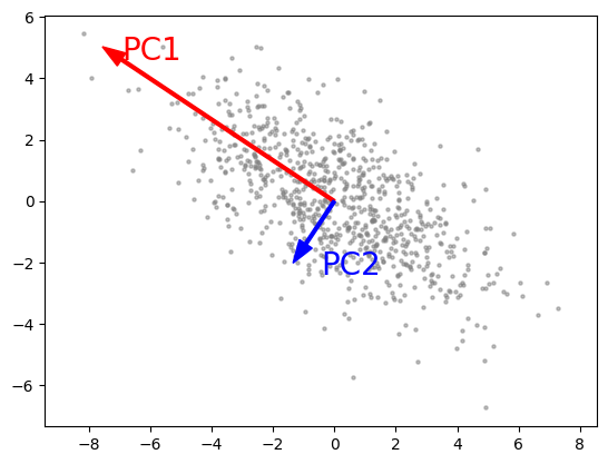
Source data:
1
2
cov = np.array([[6, -3], [-3, 3.5]])
pts = np.random.multivariate_normal([0, 0], cov, size=800)


The red arrow shows the first principal component axis (PC1) and the blue arrow shows the second principal component axis (PC2). The two axes are orthogonal.
红色箭头表示第一主成分轴（PC1），蓝色箭头表示第二主成分轴。这两个轴是正交的。

info “Interpretation of PCs”
假定为联合正态分布的一组p变量的第一主成分是由原始变量的线性组合形成的衍生变量，解释了最大的方差。第二个主成分解释了去除第一个成分的影响后剩下的最大方差，我们可以继续进行p次迭代，直到所有方差都得到解释。

Genotype PCA

Genotype PCs are often included in the association tests to correct for population stratification.

基因型PC通常包含在关联测试中，以纠正人群分层。

Here, usually, the data we use is the genotype matrix from the SNP array, and the covariance matrix used in PCA calculation is called genetic relationship matrix (GRM).

这里，通常我们使用的数据是SNP阵列中的基因型矩阵，PCA计算中使用的协方差矩阵称为遗传关系矩阵（GRM）。

GRM is first estimated using independent common SNPs and then PCA calculation is applied to this matrix to generate eigenvectors and eigenvalues.
Finally, the top $k$ eigenvectors with the largest eigenvalues are used to project the original genotypes into a new feature subspace, which has much fewer dimensions than the original one (dimension reduction).

首先使用独立的公共SNP估计GRM，然后将PCA计算应用于该矩阵以生成特征向量和特征值。
最后，使用具有最大特征值的前$k$特征向量将原始基因型投影到一个新的特征子空间中，该特征子空间的维数比原始特征子空间少得多（降维）。

info “Genetic relationship matrix (GRM)”

Citation: Yang, J., Lee, S. H., Goddard, M. E., & Visscher, P. M. (2011). GCTA: a tool for genome-wide complex trait analysis. The American Journal of Human Genetics, 88(1), 76-82.

PCA is by far the most commonly used dimension reduction approach used in population genetics which could identify the difference in ancestry among the sample individuals.

PCA是迄今为止在群体遗传学中最常用的降维方法，可以识别样本个体之间的祖先差异。

The population outliers should be excluded from the samples used in GWAS to avoid bias caused by population stratification.
For GWAS, we also need to include top PCs to adjust for the population stratification.

应将总体异常值从GWAS中使用的样本中排除，以避免由总体分层引起的偏差。
对于GWAS，我们还需要包括顶级PC，以适应人口分层。

Please read the following paper on how we apply PCA to genetic data:
Price, A., Patterson, N., Plenge, R. et al. Principal components analysis corrects for stratification in genome-wide association

请阅读以下关于我们如何将PCA应用于遗传数据的论文：
Price，A.，Patterson，N.，Plenge，R.等人。主成分分析校正了全基因组关联中的分层 studies. Nat Genet 38, 904–909 (2006). https://doi.org/10.1038/ng1847 https://www.nature.com/articles/ng1847

So before association analysis, we will learn how to run PCA analysis first.

Preparation
PCA steps
Sample codes
Plotting the PCs
PCA-UMAP
References

!!! info “Genotype PCA workflow”

Preparation

Exclude SNPs in high-LD or HLA regions

For PCA, we first exclude SNPs in high-LD or HLA regions from the genotype data.

对于PCA，我们首先从基因型数据中排除高LD或HLA区域的SNP。

!!! quote “The reason why we want to exclude such high-LD or HLA regions”
- Price, A. L., Weale, M. E., Patterson, N., Myers, S. R., Need, A. C., Shianna, K. V., Ge, D., Rotter, J. I., Torres, E., Taylor, K. D., Goldstein, D. B., & Reich, D. (2008). Long-range LD can confound genome scans in admixed populations. American journal of human genetics, 83(1), 132–139. https://doi.org/10.1016/j.ajhg.2008.06.005

Download BED-like files for high-LD or HLA regions

You can simply copy the list of high-LD or HLA regions in genome build version(.bed format) to a text file high-ld.txt.

您可以简单地将基因组构建版本（.bed格式）中的高LD或HLA区域列表复制到文本文件“high LD.txt”中。

!!! quote “High LD regions were obtained from”
https://genome.sph.umich.edu/wiki/Regions_of_high_linkage_disequilibrium_(LD)

!!! info “High LD regions of hg19”

title

1	48000000	52000000	highld
2	86000000	100500000	highld
2	134500000	138000000	highld
2	183000000	190000000	highld
3	47500000	50000000	highld
3	83500000	87000000	highld
3	89000000	97500000	highld
5	44500000	50500000	highld
5	98000000	100500000	highld
5	129000000	132000000	highld
5	135500000	138500000	highld
6	25000000	35000000	highld
6	57000000	64000000	highld
6	140000000	142500000	highld
7	55000000	66000000	highld
8	7000000 13000000	highld
8	43000000	50000000	highld
8	112000000	115000000	highld
10	37000000	43000000	highld
11	46000000	57000000	highld
11	87500000	90500000	highld
12	33000000	40000000	highld
12	109500000	112000000	highld
20	32000000	34500000	highld

Create a list of SNPs in high-LD or HLA regions

Next, use high-ld.txt to extract all SNPs that are located in the regions described in the file using the code as follows:

接下来，使用“high ld.txt”使用以下代码提取位于文件中描述的区域中的所有SNP：

1	plink --file ${plinkFile} --make-set high-ld.txt --write-set --out hild

example “Create a list of SNPs in the regions specified in high-ld.txt “

1
2
3
4
5
6
7
plinkFile="../04_Data_QC/sample_data.clean"

plink \
	--bfile ${plinkFile} \
	--make-set high-ld-hg19.txt \
	--write-set \
	--out hild


And all SNPs in the regions will be extracted to hild.set.

1
2
3
4
5
6
7
8
9
10
11
$head hild.set
highld
1:48000156:C:G
1:48002096:C:G
1:48003081:T:C
1:48004776:C:T
1:48006500:A:G
1:48006546:C:T
1:48008102:T:G
1:48009994:C:T
1:48009997:C:A

For downstream analysis, we can exclude these SNPs using --exclude hild.set.

对于下游分析，我们可以使用“–exclude hild.set”排除这些SNP。

PCA steps

info “Steps to perform a typical genomic PCA analysis”

info“执行典型基因组PCA分析的步骤”

- 1. LD-Pruning (https://www.cog-genomics.org/plink/2.0/ld#indep)
- 2. Removing relatives from calculating PCs (usually 2-degree) (https://www.cog-genomics.org/plink/2.0/distance#king_cutoff)
- 3. Running PCA using un-related samples and independent SNPs (https://www.cog-genomics.org/plink/2.0/strat#pca)
- 4. Projecting to all samples (https://www.cog-genomics.org/plink/2.0/score#pca_project)

!!! info “MAF filter for LD-pruning and PCA”
For LD-pruning and PCA, we usually only use variants with MAF > 0.01 or MAF>0.05 ( --maf 0.01 or --maf 0.05) for robust estimation.

对于LD修剪和PCA，我们通常只使用MAF>0.01或MAF>0.05（“-MAF 0.01”或“-MAF 0.05”）的变量进行稳健估计。

Sample codes

example “Sample codes for performing PCA”

plinkFile="" #please set this to your own path
outPrefix="plink_results"
threadnum=2
hildset = hild.set

#接下来，使用“high ld.txt”使用以下代码提取位于文件中描述的区域中的所有SNP：
LD-pruning, excluding high-LD and HLA regions
plink2
–bfile ${plinkFile}
–maf 0.01
–threads ${threadnum}
–exclude ${hildset} \
–indep-pairwise 500 50 0.2
–out ${outPrefix}
# Remove related samples using king-cuttoff
plink2
–bfile ${plinkFile}
–extract ${outPrefix}.prune.in
–king-cutoff 0.0884
–threads ${threadnum}
–out ${outPrefix}

# PCA after pruning and removing related samples
plink2 \
        --bfile ${plinkFile} \
        --keep ${outPrefix}.king.cutoff.in.id \
        --extract ${outPrefix}.prune.in \
        --freq counts \
        --threads ${threadnum} \
        --pca approx allele-wts 10 \     
        --out ${outPrefix}

# Projection (related and unrelated samples)
plink2 \
        --bfile ${plinkFile} \
        --threads ${threadnum} \
        --read-freq ${outPrefix}.acount \
        --score ${outPrefix}.eigenvec.allele 2 6 header-read no-mean-imputation variance-standardize \
        --score-col-nums 7-16 \
        --out ${outPrefix}_projected
1
2
3
4
5
6
7
8
9
10
11
12
13
14
15
16
17
18
19
20
21
22
23
24
25
26
27
28
29
30
31
32
33
34
35
36
37
38
39
40

info "`--pca` and `--pca approx`"
For step 3, please note that `approx` flag is only recommended for analysis of >5000 samples. (It was applied in the sample code anyway because in real analysis you usually have a much larger sample size, though the sample size of our data is just ~500)

对于步骤3，请注意“近似”标志仅建议用于分析>5000个样本。（无论如何，它都被应用于示例代码中，因为在实际分析中，你通常会有更大的样本量，尽管我们数据的样本量只有~500）

After step 3, the `allele-wts 10` modifier requests an additional one-line-per-allele `.eigenvec.allele` file with the first `10 PCs` expressed as allele weights instead of sample weights.

在步骤3之后，“`allele-wts 10` ”修饰语要求每个等位基因“.eigenvec.allele”文件额外增加一行，其中前“10个PC”表示为等位基因权重，而不是样本权重。

We will get the `plink_results.eigenvec.allele` file, which will be used to project onto all samples along with an allele count `plink_results.acount` file.

我们将得到“plink_results.eigenvec.allele”文件，该文件将与等位基因计数“plink.results.account”文件一起用于投影到所有样本上。

In the projection, `score ${outPrefix}.eigenvec.allele 2 5` sets the `ID` (2nd column) and `A1` (5th column), `score-col-nums 6-15` sets the first 10 PCs to be projected. Please check https://www.cog-genomics.org/plink/2.0/score#pca_project for more details on the projection.

在投影中，“score${outPrefix}.englenevec.allele 2 5”设置“ID”（第2列）和“A1”（第5列），“scores col nums 6-15”设置要投影的前10个PC。请检查https://www.cog-genomics.org/plink/2.0/score#pca_project有关投影的更多详细信息。

warning "Please check the content of your `.eigenvec.allele` file" 
    Using recent plink2 versions, there are some minor changes in the output format. 
    `A1` is the 6th column, and the `score-col-nums` should be `7-16`
    Please adjust the column number in your script accordingly. 

警告“请检查您的`.englenevec.alezole`文件的内容”
使用最新的plink2版本，输出格式有一些细微的变化。 
`A1`是第6列，而`score col-nums'应该是`7-16`
请相应地调整脚本中的列号。

example "Allele weight and count files"
    ```txt title="plink_results.eigenvec.allele"
    #CHROM  ID      REF     ALT     PROVISIONAL_REF?        A1      PC1     PC2     PC3     PC4     PC5     PC6     PC7PC8      PC9     PC10
    1       1:15774:G:A     G       A       Y       G       0.57834 -1.03002        0.744557        -0.161887       0.389223    -0.0514592      0.133195        -0.0336162      -0.846376       0.0542876
    1       1:15774:G:A     G       A       Y       A       -0.57834        1.03002 -0.744557       0.161887        -0.389223   0.0514592       -0.133195       0.0336162       0.846376        -0.0542876
    1       1:15777:A:G     A       G       Y       A       -0.585215       0.401872        -0.393071       -1.79583   0.89579  -0.700882       -0.103729       -0.694495       -0.007313       0.513223
    1       1:15777:A:G     A       G       Y       G       0.585215        -0.401872       0.393071        1.79583 -0.89579    0.700882        0.103729        0.694495        0.007313        -0.513223
    1       1:57292:C:T     C       T       Y       C       -0.123768       0.912046        -0.353606       -0.220148  -0.893017        -0.374505       -0.141002       -0.249335       0.625097        0.206104
    1       1:57292:C:T     C       T       Y       T       0.123768        -0.912046       0.353606        0.220148   0.893017 0.374505        0.141002        0.249335        -0.625097       -0.206104
    1       1:77874:G:A     G       A       Y       G       1.49202 -1.12567        1.19915 0.0755314       0.401134   -0.015842        0.0452086       0.273072        -0.00716098     0.237545
    1       1:77874:G:A     G       A       Y       A       -1.49202        1.12567 -1.19915        -0.0755314      -0.401134   0.015842        -0.0452086      -0.273072       0.00716098      -0.237545
    1       1:87360:C:T     C       T       Y       C       -0.191803       0.600666        -0.513208       -0.0765155 -0.656552        0.0930399       -0.0238774      -0.330449       -0.192037       -0.727729


title
1
2
3
4
5
6
7
8
9
10
#CHROM  ID      REF     ALT     PROVISIONAL_REF?        ALT_CTS OBS_CT
1       1:15774:G:A     G       A       Y       28      994
1       1:15777:A:G     A       G       Y       73      994
1       1:57292:C:T     C       T       Y       104     988
1       1:77874:G:A     G       A       Y       19      994
1       1:87360:C:T     C       T       Y       23      998
1       1:125271:C:T    C       T       Y       967     996
1       1:232449:G:A    G       A       Y       185     996
1       1:533113:A:G    A       G       Y       129     992
1       1:565697:A:G    A       G       Y       334     996

Eventually, we will get the PCA results for all samples.

最终，我们将得到所有样本的PCA结果。

!!! example “PCA results for all samples”

title

#FID    IID     ALLELE_CT       NAMED_ALLELE_DOSAGE_SUM PC1_AVG PC2_AVG PC3_AVG PC4_AVG PC5_AVG PC6_AVG PC7_AVG PC8_AVG     PC9_AVG PC10_AVG
HG00403 HG00403 390256  390256  0.00290265      -0.0248649      0.0100408       0.00957591      0.00694349      -0.00222251 0.0082228       -0.00114937     0.00335249      0.00437471
HG00404 HG00404 390696  390696  -0.000141221    -0.027965       0.025389        -0.00582538     -0.00274707     0.00658501  0.0113803       0.0077766       0.0159976       0.0178927
HG00406 HG00406 388524  388524  0.00707397      -0.0315445      -0.00437011     -0.0012621      -0.0114932      -0.00539483 -0.00620153     0.00452379      -0.000870627    -0.00227979
HG00407 HG00407 388808  388808  0.00683977      -0.025073       -0.00652723     0.00679729      -0.0116 -0.0102328 0.0139572        0.00618677      0.0138063       0.00825269
HG00409 HG00409 391646  391646  0.000398695     -0.0290334      -0.0189352      -0.00135977     0.0290436       0.00942829  -0.0171194      -0.0129637      0.0253596       0.022907
HG00410 HG00410 391600  391600  0.00277094      -0.0280021      -0.0209991      -0.00799085     0.0318038       -0.00284209 -0.031517       -0.0010026      0.0132541       0.0357565
HG00419 HG00419 387118  387118  0.00684154      -0.0326244      0.00237159      0.0167284       -0.0119737      -0.0079637  -0.0144339      0.00712756      0.0114292       0.00404426
HG00421 HG00421 387720  387720  0.00157095      -0.0338115      -0.00690541     0.0121058       0.00111378      0.00530794  -0.0017545      -0.00121793     0.00393407      0.00414204
HG00422 HG00422 387466  387466  0.00439167      -0.0332386      0.000741526     0.0124843       -0.00362248     -0.00343393 -0.00735112     0.00944759      -0.0107516      0.00376537

Plotting the PCs

You can now create scatterplots of the PCs using R or Python.

For plotting using Python:
plot_PCA.ipynb

!!! example “Scatter plot of PC1 and PC2 using 1KG EAS individuals”

Note : We only used a small proportion of all available variants. This figure only very roughly shows the population structure in East Asia.

Requirements:

python>3
numpy,pandas,seaborn,matplotlib

PCA-UMAP

(optional)
We can also apply another non-linear dimension reduction algorithm called UMAP to the PCs to further identify the local structures. (PCA-UMAP)

我们还可以将另一种称为UMAP的非线性降维算法应用于PC，以进一步识别局部结构。（PCA-UMAP）

For more details, please check:

https://umap-learn.readthedocs.io/en/latest/index.html

An example of PCA and PCA-UMAP for population genetics:

Sakaue, S., Hirata, J., Kanai, M., Suzuki, K., Akiyama, M., Lai Too, C., … & Okada, Y. (2020). Dimensionality reduction reveals fine-scale structure in the Japanese population with consequences for polygenic risk prediction. Nature communications, 11(1), 1-11.

可视化代码

import package

1
2
3

import pandas as pd
import matplotlib.pyplot as plt
import seaborn as sns

loading files

1 2	pca = pd.read_table("../05_PCA/plink_results_projected.sscore",sep="\t") pca

	#FID	IID	ALLELE_CT	NAMED_ALLELE_DOSAGE_SUM	PC1_AVG	PC2_AVG	PC3_AVG	PC4_AVG	PC5_AVG	PC6_AVG	PC7_AVG	PC8_AVG	PC9_AVG	PC10_AVG
0	HG00403	HG00403	390256	390256	0.002903	0.024865	-0.010041	-0.009576	-0.006944	-0.002231	0.008223	0.001144	0.003275	-0.004409
1	HG00404	HG00404	390696	390696	-0.000141	0.027965	-0.025389	0.005826	0.002754	0.006582	0.011364	-0.007764	0.015910	-0.017907
2	HG00406	HG00406	388524	388524	0.007074	0.031545	0.004370	0.001262	0.011488	-0.005377	-0.006199	-0.004531	-0.000890	0.002100
3	HG00407	HG00407	388808	388808	0.006840	0.025073	0.006527	-0.006797	0.011606	-0.010235	0.013986	-0.006156	0.013815	-0.008209
4	HG00409	HG00409	391646	391646	0.000399	0.029033	0.018935	0.001360	-0.029035	0.009427	-0.017172	0.012989	0.025203	-0.022907
...	...	...	...	...	...	...	...	...	...	...	...	...	...	...
495	NA19087	NA19087	390232	390232	-0.082261	-0.033163	-0.045499	0.011398	-0.000029	-0.006535	0.012385	0.006725	-0.016496	-0.023087
496	NA19088	NA19088	391510	391510	-0.087183	-0.043433	-0.040188	-0.003610	0.000164	0.002310	0.000112	-0.007414	-0.011923	-0.007827
497	NA19089	NA19089	391462	391462	-0.084082	-0.036118	0.036355	-0.008738	0.037525	0.004119	0.008640	0.000592	-0.001666	-0.015841
498	NA19090	NA19090	392880	392880	-0.073580	-0.026163	0.032193	-0.006599	0.039057	0.000708	0.012244	0.000480	-0.000231	0.031587
499	NA19091	NA19091	389664	389664	-0.081632	-0.041455	0.032200	-0.003717	0.046710	0.015204	0.003151	0.004921	-0.001610	0.021045

500 rows × 14 columns

1 2	ped = pd.read_table("../01_Dataset/integrated_call_samples_v3.20130502.ALL.panel",sep="\t") ped

	sample	pop	super_pop	gender	Unnamed: 4	Unnamed: 5
0	HG00096	GBR	EUR	male	NaN	NaN
1	HG00097	GBR	EUR	female	NaN	NaN
2	HG00099	GBR	EUR	female	NaN	NaN
3	HG00100	GBR	EUR	female	NaN	NaN
4	HG00101	GBR	EUR	male	NaN	NaN
...	...	...	...	...	...	...
2499	NA21137	GIH	SAS	female	NaN	NaN
2500	NA21141	GIH	SAS	female	NaN	NaN
2501	NA21142	GIH	SAS	female	NaN	NaN
2502	NA21143	GIH	SAS	female	NaN	NaN
2503	NA21144	GIH	SAS	female	NaN	NaN

2504 rows × 6 columns

### Merge PCA and population information

1 2	pcaped=pd.merge(pca,ped,right_on="sample",left_on="IID",how="inner") pcaped

	#FID	IID	ALLELE_CT	NAMED_ALLELE_DOSAGE_SUM	PC1_AVG	PC2_AVG	PC3_AVG	PC4_AVG	PC5_AVG	PC6_AVG	PC7_AVG	PC8_AVG	PC9_AVG	PC10_AVG	sample	pop	super_pop	gender	Unnamed: 4	Unnamed: 5
0	HG00403	HG00403	390256	390256	0.002903	0.024865	-0.010041	-0.009576	-0.006944	-0.002231	0.008223	0.001144	0.003275	-0.004409	HG00403	CHS	EAS	male	NaN	NaN
1	HG00404	HG00404	390696	390696	-0.000141	0.027965	-0.025389	0.005826	0.002754	0.006582	0.011364	-0.007764	0.015910	-0.017907	HG00404	CHS	EAS	female	NaN	NaN
2	HG00406	HG00406	388524	388524	0.007074	0.031545	0.004370	0.001262	0.011488	-0.005377	-0.006199	-0.004531	-0.000890	0.002100	HG00406	CHS	EAS	male	NaN	NaN
3	HG00407	HG00407	388808	388808	0.006840	0.025073	0.006527	-0.006797	0.011606	-0.010235	0.013986	-0.006156	0.013815	-0.008209	HG00407	CHS	EAS	female	NaN	NaN
4	HG00409	HG00409	391646	391646	0.000399	0.029033	0.018935	0.001360	-0.029035	0.009427	-0.017172	0.012989	0.025203	-0.022907	HG00409	CHS	EAS	male	NaN	NaN
...	...	...	...	...	...	...	...	...	...	...	...	...	...	...	...	...	...	...	...	...
495	NA19087	NA19087	390232	390232	-0.082261	-0.033163	-0.045499	0.011398	-0.000029	-0.006535	0.012385	0.006725	-0.016496	-0.023087	NA19087	JPT	EAS	female	NaN	NaN
496	NA19088	NA19088	391510	391510	-0.087183	-0.043433	-0.040188	-0.003610	0.000164	0.002310	0.000112	-0.007414	-0.011923	-0.007827	NA19088	JPT	EAS	male	NaN	NaN
497	NA19089	NA19089	391462	391462	-0.084082	-0.036118	0.036355	-0.008738	0.037525	0.004119	0.008640	0.000592	-0.001666	-0.015841	NA19089	JPT	EAS	male	NaN	NaN
498	NA19090	NA19090	392880	392880	-0.073580	-0.026163	0.032193	-0.006599	0.039057	0.000708	0.012244	0.000480	-0.000231	0.031587	NA19090	JPT	EAS	female	NaN	NaN
499	NA19091	NA19091	389664	389664	-0.081632	-0.041455	0.032200	-0.003717	0.046710	0.015204	0.003151	0.004921	-0.001610	0.021045	NA19091	JPT	EAS	male	NaN	NaN

500 rows × 20 columns

Plotting

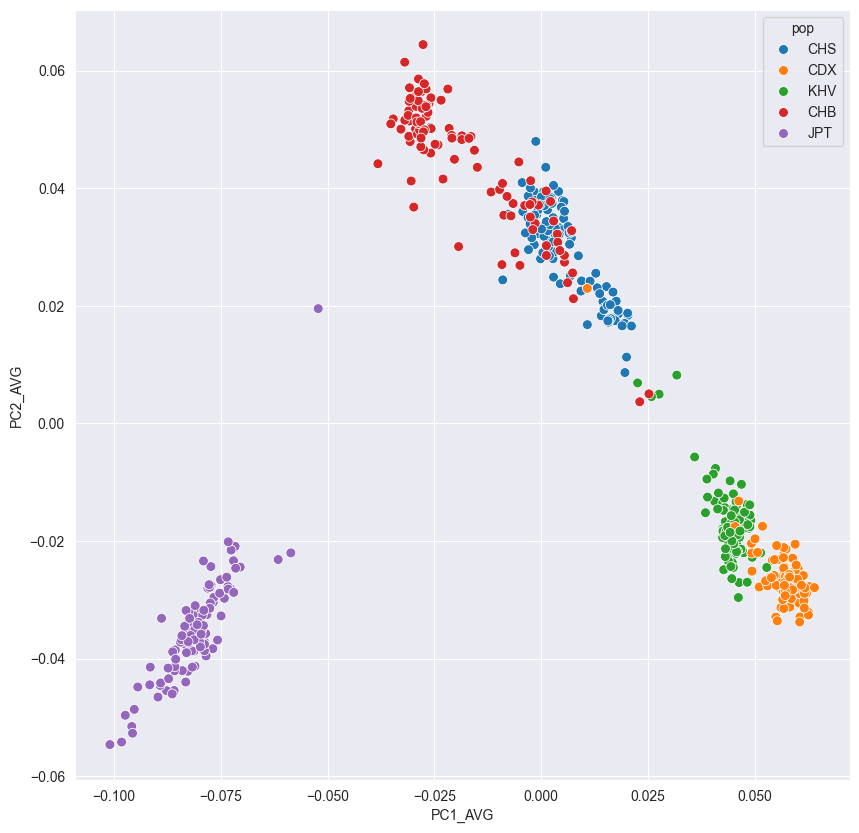
1 2	plt.figure(figsize=(10,10)) sns.scatterplot(data=pcaped,x="PC1_AVG",y="PC2_AVG",hue="pop",s=50)

pca—in—aisan—distribution

日本东京群体(Japanese in Tokyo, JPT)、北京汉族(Han Chinese in Beijing, CHB)、南方汉族(Southern Han Chinese, CHS)、西双版纳傣族(Chinese Dai in Xishuangbanna, CDX)、越南京族(Kinh in Ho Chi Minh City, KHV)

这样的分布图是可以画出很多张的，实际上都是东亚部分

References

(PCA) Price, A., Patterson, N., Plenge, R. et al. Principal components analysis corrects for stratification in genome-wide association studies. Nat Genet 38, 904–909 (2006). https://doi.org/10.1038/ng1847 https://www.nature.com/articles/ng1847
(why removing high-LD regions) Price, A. L., Weale, M. E., Patterson, N., Myers, S. R., Need, A. C., Shianna, K. V., Ge, D., Rotter, J. I., Torres, E., Taylor, K. D., Goldstein, D. B., & Reich, D. (2008). Long-range LD can confound genome scans in admixed populations. American journal of human genetics, 83(1), 132–139. https://doi.org/10.1016/j.ajhg.2008.06.005
(UMAP) McInnes, L., Healy, J., & Melville, J. (2018). Umap: Uniform manifold approximation and projection for dimension reduction. arXiv preprint arXiv:1802.03426.
(UMAP in population genetics) Diaz-Papkovich, A., Anderson-Trocmé, L. & Gravel, S. A review of UMAP in population genetics. J Hum Genet 66, 85–91 (2021). https://doi.org/10.1038/s10038-020-00851-4 https://www.nature.com/articles/s10038-020-00851-4
(king-cutoff) Manichaikul, A., Mychaleckyj, J. C., Rich, S. S., Daly, K., Sale, M., & Chen, W. M. (2010). Robust relationship inference in genome-wide association studies. Bioinformatics, 26(22), 2867-2873.