PLINK工具用于数据的质量控制QC
PLINK basics(PLINK基础)
In this module, we will learn the basics of genotype data QC using PLINK, which is one of the most commonly used software in complex trait genomics. (Huge thanks to the developers: PLINK1.9 and PLINK2)用PLINK解决基因数据的质量控制问题
Table of Contents
- Preparation
- PLINK tutorial
- Calculate the missing rate and call rate
- Calculate allele frequency
- Hardy-Weinberg equilibrium exact test
- Applying filters
- LD-Pruning
- Calculate the inbreeding F coefficient
- Sample & SNP filtering (extract/exclude/keep/remove)
- LD calculation
- Estimate IBD / PI_HAT
- Data management (make-bed/recode)
- Apply all the filters to obtain a clean dataset
- Other common QC steps not included in this tutorial
- Exercise
- Additional resources
- Reference
Preparation
PLINK 1.9&2 installation
To get prepared for genotype QC, we will need to make directories, download software and add the software to your environment path.
First, we will simply create some directories to keep the tools we need to use.
先建立一个对应的存储PLINK文件的文件架构
example “Create directories”
1 | cd ~ |

You can download each tool into its corresponding directories.
The bin directory here is for keeping all the symbolic links to the executable files of each tool.
In this way, it is much easier to manage and organize the paths and tools. We will only add the bin directory here to the environment path.
Download PLINK1.9 and PLINK2 and then unzip
Next, go to the Plink webpage to download the software. We will need both PLINK1.9 and PLINK2.
Download PLINK1.9 and PLINK2 from the following webpage to the corresponding directories:
- PLINK1.9 : https://www.cog-genomics.org/plink/
- PLINK2 : https://www.cog-genomics.org/plink/2.0/
!!! info
If you are using Mac or Windows, then please download the Mac or Windows version. In this tutorial, we will use a Linux system and the Linux version of PLINK.
Find the suitable version on the PLINK website, right-click and copy the link address.
example “Download PLINK2 (Linux AVX2 AMD)”
1 | cd ~/tools/plink2 |
Then do the same for PLINK1.9
example “Download PLINK1.9 (Linux 64-bit)”
1 | cd ~/tools/plink |
Create symbolic links
After downloading and unzipping, we will create symbolic links for the plink binary files, and then move the link to ~/tools/bin/.
example “Create symbolic links”
创建符号链接(linux)
1 | cd ~ |
//下载解压,在windows我采取的不是建立符号链接,而是进行复制内容使对应的1.9和2.0的全部文件都出现在对应的tools/bin中
Add paths to the environment path
Then add ~/tools/bin/ to the environment path.
example
1 | export PATH=$PATH:~/tools/bin/ |
All done. Let’s test if we installed PLINK successfully or not.linux中可以使用
example “Check if PLINK is installed successfully.”
1 | plink |
Well done. We have successfully installed plink1.9 and plink2.
Download genotype data
Next, we need to download the sample genotype data. The way to create the sample data is described [here].(https://cloufield.github.io/GWASTutorial/01_Dataset/)
This dataset contains 504 EAS individuals from 1000 Genome Project Phase 3v5 with around 1 million variants.
该数据集包含来自1000基因组计划第3v5阶段的504个EAS个体,约有100万个变异。
Simply run download_sampledata.sh in 01_Dataset to download this dataset (from Dropbox). See here
warning “Sample dataset is currently hosted on Dropbox which may not be accessible for users in certain regions.”
example “Download sample data”
1 | ```bash |
不用下载,github中的文件就有
PLINK tutorial PLINK教程
Detailed descriptions can be found on plink’s website: PLINK1.9 and PLINK2.
The functions we will learn in this tutorial:
Calculating missing rate (call rate)
计算丢失率(呼叫率)
Calculating allele Frequency 计算等位基因频率
Conducting Hardy-Weinberg equilibrium exact test 进行Hardy-Weinberg平衡精确检验
Applying filters 应用过滤器
Conducting LD-Pruning 进行LD修剪
Calculating inbreeding F coefficient 近亲繁殖F系数的计算
Conducting sample & SNP filtering (extract/exclude/keep/remove) 进行样本和SNP过滤(提取/排除/保留/删除)
Estimating IBD / PI_HAT 估算IBD/PI_HAT
Calculating LD 计算LD
Data management (make-bed/recode) 数据管理(整理/重新编码)
All sample codes and results for this module are available in ./04_data_QC
QC样例
1 |
|
QC Step Summary
info “QC Step Summary”
|QC step|Option in PLINK|Commonly used threshold to exclude|
|-|-|-|
|SNP missing rate| --geno, --missing | missing rate > 0.01 (0.02, or 0.05) |
|Sample missing rate| --mind, --missing | missing rate > 0.01 (0.02, or 0.05) |
|Minor allele frequency| --freq, --maf |maf < 0.01|
|Sample Relatedness| --genome |pi_hat > 0.2 to exclude second-degree relatives|
|Hardy-Weinberg equilibrium| --hwe,--hardy|hwe < 1e-6|
|Inbreeding F coefficient|--het|outside of 3 SD from the mean|
First, we can calculate some basic statistics of our simulated data:
Missing rate (call rate)
The first thing we want to know is the missing rate of our data. Usually, we need to check the missing rate of samples and SNPs to decide a threshold to exclude low-quality samples and SNPs. (https://www.cog-genomics.org/plink/1.9/basic_stats#missing)
Sample missing rate: the proportion of missing values for an individual across all SNPs.
一个个体在所有的SNP中有几成的SNP是不存在的,假设对应的一个个体的SNP的种类数太少,那么对应的这个个体就不具备研究价值
SNP missing rate: the proportion of missing values for a SNP across all samples.
同样的一个SNP在众多的个体中的存在的频率很小证明这样的数据也没有价值
!!! info “Missing rate and Call rate”
1 | Suppose we have N samples and M SNPs for each sample. |
The input is PLINK bed/bim/fam file. Usually, they have the same prefix, and we just need to pass the prefix to --bfile option.
输入是PLINK bed/bim/fam文件。通常,它们具有相同的前缀,我们只需要将前缀传递给--bfile选项。
###PLINK语法
PLINK syntax
info “PLINK syntax”

To calculate the missing rate, we need the flag --missing, which tells PLINK to calculate the missing rate in the dataset specified by --bfile.
为了计算丢失率,我们需要标志“–missing”,它告诉PLINK计算由“–bfile”指定的数据集中的丢失率。
example “Calculate missing rate”
1 | ```bash |
This code will generate two files plink_results.imiss and plink_results.lmiss, which contain the missing rate information for samples and SNPs respectively.
分别计算缺失信息
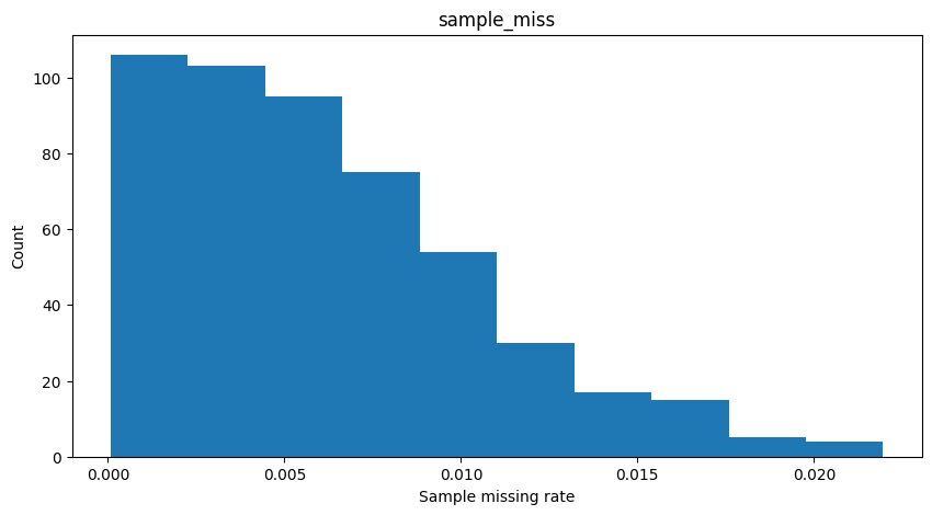
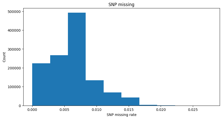
Take a look at the .imiss file. The last column shows the missing rate for samples. Since we used part of the 1000 Genome Project data this time, there are no missing SNPs in the original datasets. But for educational purposes, we randomly make some of the genotypes missing.
随机遗漏了部分SNP
1 | # missing rate for each sample |
1 | # missing rate for each SNP |
example “Distribution of sample missing rate and SNP missing rate”
1 | Note: The missing values were simulated based on normal distributions for each individual. 根据每个个体的正态分布模拟缺失值。 |
For the meaning of headers, please refer to PLINK documents.
Allele Frequency 等位基因频率
One of the most important statistics of SNPs is their frequency in a certain population. Many downstream analyses are based on investigating differences in allele frequencies.
SNP最重要的统计数据之一是它们在特定人群中的频率。许多下游分析都是基于对等位基因频率差异的调查。等位基因是指位于同源染色体上同一基因座的不同形式基因,控制同一性状的表现。
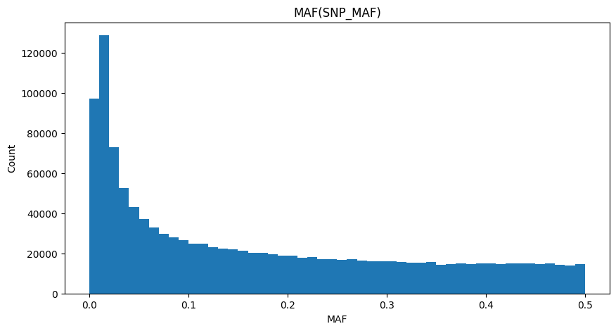
Usually, variants can be categorized into 3 groups based on their Minor Allele Frequency (MAF):
通常,变异可以根据其次要等位基因频率(MAF)分为3组:
- Common variants : MAF>=0.05 一般的
- Low-frequency variants : 0.01<=MAF<0.05 低频率
- Rare variants : MAF<0.01 罕见的
info “How to calculate Minor Allele Frequency (MAF)”
Suppose the reference allele(REF) is A and the alternative allele(ALT) is B for a certain SNP. The posible genotypes are AA, AB and BB. In a population of N samples (2N alleles),

For different downstream analyses, we might use different sets of variants. For example, for PCA, we might use only common variants. For gene-based tests, we might use only rare variants.
对于不同的下游分析,我们可能会使用不同的变量集。例如,对于PCA,我们可能只使用常见的变体。对于基于基因的检测,我们可能只使用罕见的变异。
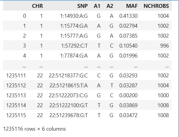
Using PLINK1.9 we can easily calculate the MAF of variants in the input data.
example “Calculate the MAF of variants using PLINK1.9”
1
2
3
4
plink \
--bfile ${genotypeFile} \
--freq \
--out plink_results
1
2
3
4
5
6
7
8
9
10
11
12
# results from plink1.9
head plink_results.frq
CHR SNP A1 A2 MAF NCHROBS
1 1:14930:A:G G A 0.4133 1004
1 1:15774:G:A A G 0.02794 1002
1 1:15777:A:G G A 0.07385 1002
1 1:57292:C:T T C 0.1054 996
1 1:77874:G:A A G 0.01996 1002
1 1:87360:C:T T C 0.02286 1006
1 1:92917:T:A A T 0.003018 994
1 1:104186:T:C T C 0.499 1002
1 1:125271:C:T C T 0.03088 1004
Next, we use plink2 to run the same options to check the difference between the results.
变异一般是小概率事件,所以对应的SNP的MAF概率会小于50%
example “Calculate the alternative allele frequencies of variants using PLINK2”
1
2
3
4
plink2 \
--bfile ${genotypeFile} \
--freq \
--out plink_results
1
2
3
4
5
6
7
8
9
10
11
12
13
14
# results from plink2
head plink_results.afreq
REF原有基因待变化碱基 ALT变异基因变化后碱基
胞嘧啶(C)、鸟嘌呤(G)、腺嘌呤(A)、胸腺嘧啶(T)和尿嘧啶(U)
#CHROM ID REF ALT PROVISIONAL_REF? ALT_FREQS OBS_CT
1 1:14930:A:G A G Y 0.413347 1004
1 1:15774:G:A G A Y 0.0279441 1002
1 1:15777:A:G A G Y 0.0738523 1002
1 1:57292:C:T C T Y 0.105422 996
1 1:77874:G:A G A Y 0.0199601 1002
1 1:87360:C:T C T Y 0.0228628 1006
1 1:92917:T:A T A Y 0.00301811 994
1 1:104186:T:C T C Y 0.500998 1002
1 1:125271:C:T C T Y 0.969124 1004
We need to pay attention to the concepts here.
In PLINK1.9, the concept here is minor (A1) and major(A2) allele, while in PLINK2 it is the reference (REF) allele and the alternative (ALT) allele.
在PLINK1.9中,这里的概念是次要(A1)和主要(A2)等位基因,而在PLINK2中,它是参考(REF)等位和替代(ALT)等位。
Major / Minor: Major allele and minor allele are defined as the allele with the highest and lower(or the second highest for multiallelic variants) allele in a given population, respectively. So major and minor alleles for a certain SNP might be different in two independent populations. The range for MAF(minor allele frequencies) is [0,0.5].
主要/次要:主要等位基因和次要等位基因分别被定义为给定人群中具有最高和较低(或多等位基因变体的第二高)等位基因的等位基因。因此,在两个独立的群体中,某个SNP的主要和次要等位基因可能不同。MAF(次要等位基因频率)的范围为[0,0.5]。
Ref / Alt: The reference (REF) and alternative (ALT) alleles are simply determined by the allele on a reference genome. If we use the same reference genome, the reference(REF) and alternative(ALT) alleles will be the same across populations. The reference allele could be major or minor in different populations. The range for alternative allele frequency is [0,1], since it could be the major allele or the minor allele in a given population.
Ref/Alt:参考(Ref)和替代(Alt)等位基因仅由参考基因组上的等位基因决定。如果我们使用相同的参考基因组,参考(REF)和替代(ALT)等位基因在人群中将是相同的。参考等位基因在不同人群中可能是主要的或次要的。替代等位基因频率的范围为[0,1],因为它可能是给定人群中的主要等位基因或次要等位基因。(在这样的评价体系中,不去计算比较小的部分)有的SNP的变化概率是超过1/2的
Hardy-Weinberg equilibrium exact test
Hardy-Weinberg平衡精确检验
For SNP QC, besides checking the missing rate, we also need to check if the SNP is in Hardy-Weinberg equilibrium:
对于SNP QC,除了检查缺失率外,我们还需要检查SNP是否处于Hardy-Weinberg平衡状态:
--hardy will perform Hardy-Weinberg equilibrium exact test for each variant. Variants with low P value usually suggest genotyping errors, or indicate evolutionary selection for these variants.
将对每种变体进行Hardy-Weinberg平衡精确检验。P值低的变异通常表明基因分型错误,或表明这些变异的进化选择。
The following command can calculate the Hardy-Weinberg equilibrium exact test statistics for all SNPs. (https://www.cog-genomics.org/plink/1.9/basic_stats#hardy)
info
Suppose we have N unrelated samples (2N alleles).
Under HWE, the exact probability of observing 
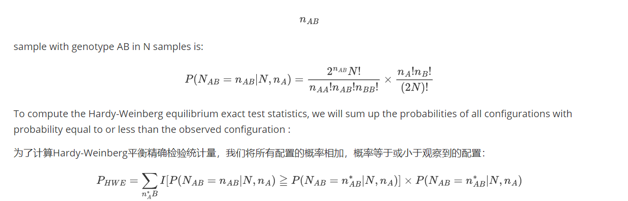
 is the indicator function. If x is true, $I(x) = 1$; otherwise, $I(x) = 0$.
Reference : Wigginton, J. E., Cutler, D. J., & Abecasis, G. R. (2005). A note on exact tests of Hardy-Weinberg equilibrium. The American Journal of Human Genetics, 76(5), 887-893. Link
example “Calculate the Hardy-Weinberg equilibrium exact test statistics for a single SNP using Python”
示例“使用Python计算单个SNP的Hardy-Weinberg平衡精确检验统计量”
This code is converted from here (Jeremy McRae) to python. Orginal citation: Wigginton, JE, Cutler, DJ, and Abecasis, GR (2005) A Note on Exact Tests of Hardy-Weinberg Equilibrium. AJHG 76: 887-893
1 |
|
example “Calculate the Hardy-Weinberg equilibrium exact test statistics using PLINK”
1 | ```bash |
head plink_results.hwe
CHR SNP TEST A1 A2 GENO O(HET) E(HET) P
1 1:14930:A:G ALL(NP) G A 4/407/91 0.8108 0.485 4.864e-61
1 1:15774:G:A ALL(NP) A G 0/28/473 0.05589 0.05433 1
1 1:15777:A:G ALL(NP) G A 1/72/428 0.1437 0.1368 0.5053
1 1:57292:C:T ALL(NP) T C 3/99/396 0.1988 0.1886 0.3393
1 1:77874:G:A ALL(NP) A G 0/20/481 0.03992 0.03912 1
1 1:87360:C:T ALL(NP) T C 0/23/480 0.04573 0.04468 1
1 1:92917:T:A ALL(NP) A T 0/3/494 0.006036 0.006018 1
1 1:104186:T:C ALL(NP) T C 74/352/75 0.7026 0.5 6.418e-20
1 1:125271:C:T ALL(NP) C T 1/29/472 0.05777 0.05985 0.3798
Applying filters
Previously we calculated the basic statistics using PLINK. But when performing certain analyses, we just want to exclude the bad-quality samples or SNPs instead of calculating the statistics for all samples and SNPs.
之前我们使用PLINK计算基本统计数据。但在进行某些分析时,我们只想排除质量差的样本或SNP,而不是计算所有样本和SNP的统计数据。
In this case we can apply the following filters for example:
--maf 0.01: exlcude snps with maf<0.01(突变或者不突变的概率太小,这样的SNP变异不可取)--geno 0.02:filters out all variants with missing rates exceeding 0.02(SNP在个体中出现的不够普遍这样的snp不可取)--mind 0.02:filters out all samples with missing rates exceeding 0.02(个体的变异的SNP包含的太少,也是不允许的)--hwe 1e-6: filters out all variants which have Hardy-Weinberg equilibrium exact test p-value below the provided threshold. NOTE: With case/control data, cases and missing phenotypes are normally ignored.筛选出Hardy-Weinberg平衡精确检验p值低于所提供阈值的所有变体。注:对于病例/对照数据,病例和缺失表型通常被忽略。 (see https://www.cog-genomics.org/plink/1.9/filter#hwe)
We will apply these filters in the following example if LD-pruning.
在以下示例中,我们将应用这些过滤器进行LD修剪。
LD Pruning
There is often strong Linkage disequilibrium(LD) among SNPs, for some analysis we don’t need all SNPs and we need to remove the redundant SNPs to avoid bias in genetic estimations. For example, for relatedness estimation, we will use only LD-Pruned SNP set.
SNP之间通常存在很强的连锁不平衡(LD),对于某些分析,我们不需要所有SNP,我们需要删除冗余的SNP以避免遗传估计中的偏差。例如,对于相关性估计,我们将仅使用LD修剪的SNP集。
We can use --indep-pairwise 50 5 0.2 to filter out those in strong LD and keep only the independent SNPs.
info “Meaning of --indep-pairwise x y z“
- consider a window of `x` SNPs
- calculate LD between each pair of SNPs in the window and remove one of a pair of SNPs if the LD is greater than `z`
- shift the window `y` SNPs forward and repeat the procedure.
Please check https://www.cog-genomics.org/plink/1.9/ld#indep for details.
Combined with the filters we just introduced, we can run:
example
1
2
3
4
5
6
7
8plink \
--bfile ${genotypeFile} \
--maf 0.01 \
--geno 0.02 \
--mind 0.02 \
--hwe 1e-6 \
--indep-pairwise 50 5 0.2 \
--out plink_results
This command generates two outputs: plink_results.prune.in and plink_results.prune.out
plink_results.prune.in is the independent set of SNPs we will use in the following analysis.
You can check the PLINK log for how many variants were removed based on the filters you applied:
1
2
3
4
5
6
Total genotyping rate in remaining samples is 0.993916.
108837 variants removed due to missing genotype data (--geno).
--hwe: 9754 variants removed due to Hardy-Weinberg exact test.
87149 variants removed due to minor allele threshold(s)
(--maf/--max-maf/--mac/--max-mac).
1029376 variants and 501 people pass filters and QC.
Let's take a look at the LD-pruned SNP file. Basically, it just contains one SNP id per line.
1
2
3
4
5
6
7
8
9
10
11
head plink_results.prune.in
1:15774:G:A
1:15777:A:G
1:77874:G:A
1:87360:C:T
1:125271:C:T
1:232449:G:A
1:533113:A:G
1:565697:A:G
1:566933:A:G
1:567092:T:C
Inbreeding F coefficient
Next, we can check the heterozygosity F of samples (https://www.cog-genomics.org/plink/1.9/basic_stats#ibc) :
-het option will compute observed and expected autosomal homozygous genotype counts for each sample. Usually, we need to exclude individuals with high or low heterozygosity coefficients, which suggests that the sample might be contaminated.
选项将计算每个样本的观察到的和预期的常染色体纯合基因型计数。通常,我们需要排除杂合度系数高或低的个体,这表明样本可能被污染。
info “Inbreeding F coefficient calculation by PLINK”
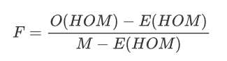
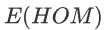 :Expected Homozygous Genotype Count
  :Observed Homozygous Genotype Count
 - M : Number of SNPs
High F may indicate a relatively high level of inbreeding.
高F可能表明近亲繁殖水平相对较高。
Low F may suggest the sample DNA was contaminated.
低F可能表明样本DNA被污染。
warning “Performing LD-pruning beforehand since these calculations do not take LD into account.”
警告“预先执行LD修剪,因为这些计算不考虑LD。”
example “Calculate inbreeding F coefficient” 示例“计算近亲繁殖F系数”
1
2
3
4
5
plink \
--bfile ${genotypeFile} \
--extract plink_results.prune.in \
--het \
--out plink_results
Check the output:
1
2
3
4
5
6
7
8
9
10
11
head plink_results.het
FID IID O(HOM) E(HOM) N(NM) F
HG00403 HG00403 180222 1.796e+05 217363 0.01698
HG00404 HG00404 180127 1.797e+05 217553 0.01023
HG00406 HG00406 178891 1.789e+05 216533 -0.0001138
HG00407 HG00407 178992 1.79e+05 216677 -0.0008034
HG00409 HG00409 179918 1.801e+05 218045 -0.006049
HG00410 HG00410 179782 1.801e+05 218028 -0.009268
HG00419 HG00419 178362 1.783e+05 215849 0.001315
HG00421 HG00421 178222 1.785e+05 216110 -0.008288
HG00422 HG00422 178316 1.784e+05 215938 -0.0022
A commonly used method is to exclude samples with heterozygosity F deviating more than 3 standard deviations (SD) from the mean. Some studies used a fixed value such as +-0.15 or +-0.2.
warning “Usually we will use only LD-pruned SNPs for the calculation of F.”
We can plot the distribution of F:
example “Distribution of $F_{het}$ in sample data”
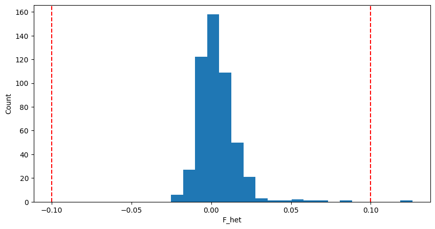
Here we use +-0.1 as the  threshold for convenience.
为了方便起见,这里我们使用+-0.1作为
example “Create sample list of individuals with extreme F using awk”
示例“使用awk创建具有极端F的个人示例列表”
1 | ``` |
Sample & SNP filtering (extract/exclude/keep/remove)
Sometimes we will use only a subset of samples or SNPs included the original dataset.
In this case, we can use --extract or --exclude to select or exclude SNPs from analysis, --keep or --remove to select or exclude samples.
有时我们只会使用原始数据集中包含的样本或SNP的子集。
在这种情况下,我们可以使用“–extract”或“–exclude”从分析中选择或排除SNP,使用“–keep”或“–remove”选择或排除样本。
For --keep or --remove, the input is the filename of a sample FID and IID file.
For --extract or --exclude, the input is the filename of an SNP list file.
1 | head plink_results.prune.in |
IBD / PI_HAT / kinship coefficient(共祖血缘系数)
--genome will estimate IBS/IBD. Usually, for this analysis, we need to prune our data first since the strong LD will cause bias in the results.
将估计IBS/IBD。通常,对于这种分析,我们需要首先修剪我们的数据,因为强LD会导致结果出现偏差。(此步骤计算量很大)
Combined with the --extract, we can run:
info “How PLINK estimates IBD”
信息“PLINK如何估计IBD”
The prior probability of IBS sharing can be modeled as:
IBS共享的先验概率可以建模为: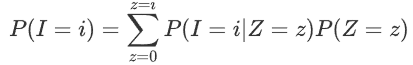
- I: IBS state (I = 0, 1, or 2)
- Z: IBD state (Z = 0, 1, or 2)
 是等位基因频率的函数。PLINK将对所有SNP进行平均,以获得
So the proportion of alleles shared IBD ( ) can be estimated by:

example “Estimate IBD”
1
2
3
4
5plink \
--bfile ${genotypeFile} \
--extract plink_results.prune.in \
--genome \
--out plink_results
PI_HAT is the IBD estimation. Please check https://www.cog-genomics.org/plink/1.9/ibd for more details.
1
2
3
4
5
6
7
8
9
10
11
head plink_results.genome
FID1 IID1 FID2 IID2 RT EZ Z0 Z1 Z2 PI_HAT PHE DST PPC RATIO
HG00403 HG00403 HG00404 HG00404 UN NA 1.0000 0.0000 0.0000 0.0000 -1 0.858562 0.3679 1.9774
HG00403 HG00403 HG00406 HG00406 UN NA 0.9805 0.0044 0.0151 0.0173 -1 0.858324 0.8183 2.0625
HG00403 HG00403 HG00407 HG00407 UN NA 0.9790 0.0000 0.0210 0.0210 -1 0.857794 0.8034 2.0587
HG00403 HG00403 HG00409 HG00409 UN NA 0.9912 0.0000 0.0088 0.0088 -1 0.857024 0.2637 1.9578
HG00403 HG00403 HG00410 HG00410 UN NA 0.9699 0.0235 0.0066 0.0184 -1 0.858194 0.6889 2.0335
HG00403 HG00403 HG00419 HG00419 UN NA 1.0000 0.0000 0.0000 0.0000 -1 0.857643 0.8597 2.0745
HG00403 HG00403 HG00421 HG00421 UN NA 0.9773 0.0218 0.0010 0.0118 -1 0.857276 0.2186 1.9484
HG00403 HG00403 HG00422 HG00422 UN NA 0.9880 0.0000 0.0120 0.0120 -1 0.857224 0.8277 2.0652
HG00403 HG00403 HG00428 HG00428 UN NA 0.9801 0.0069 0.0130 0.0164 -1 0.858162 0.9812 2.1471
info “KING-robust kinship estimator”
PLINK2 uses KING-robust kinship estimator, which is more robust in the presence of population substructure. See [here](https://www.cog-genomics.org/plink/2.0/distance#make_king).
Manichaikul, A., Mychaleckyj, J. C., Rich, S. S., Daly, K., Sale, M., & Chen, W. M. (2010). Robust relationship inference in genome-wide association studies. Bioinformatics, 26(22), 2867-2873.
Since the samples are unrelated, we do not need to remove any samples at this step. But remember to check this for your dataset.
LD calculation
We can also use our data to estimate the LD between a pair of SNPs.
我们还可以使用我们的数据来估计一对SNP之间的LD。
info “Details on LD can be found here“
--chr option in PLINK allows us to include SNPs on a specific chromosome.
To calculate LD r2 for SNPs on chr22 , we can run:
PLINK中的选项允许我们在特定染色体上包含SNP。
为了计算chr22上SNP的LD r2,我们可以运行:
!!! example Calculate LD r2 for SNPs on chr22
1
2
3
4
5
plink \
--bfile ${genotypeFile} \
--chr 22 \
--r2 \
--out plink_results
1
2
3
4
5
6
7
8
9
10
11
head plink_results.ld
CHR_A BP_A SNP_A CHR_B BP_B SNP_B R2
22 16069141 22:16069141:C:G 22 16071624 22:16071624:A:G 0.771226
22 16069784 22:16069784:A:T 22 16149743 22:16149743:T:A 0.217197
22 16069784 22:16069784:A:T 22 16150589 22:16150589:C:A 0.224992
22 16069784 22:16069784:A:T 22 16159060 22:16159060:G:A 0.2289
22 16149743 22:16149743:T:A 22 16150589 22:16150589:C:A 0.965109
22 16149743 22:16149743:T:A 22 16152606 22:16152606:T:C 0.692157
22 16149743 22:16149743:T:A 22 16159060 22:16159060:G:A 0.721796
22 16149743 22:16149743:T:A 22 16193549 22:16193549:C:T 0.336477
22 16149743 22:16149743:T:A 22 16212542 22:16212542:C:T 0.442424
Data management (make-bed/recode)
By far the input data we use is in binary form, but sometimes we may want the text version.
到目前为止,我们使用的输入数据是二进制形式的,但有时我们可能需要文本版本。
!!! info Format conversion

To convert the formats, we can run:
要转换格式,我们可以运行:
example “Convert PLINK formats”
1
2
3
4
5
6
7
8
9
10
11
12
#extract the 1000 samples with the pruned SNPs, and make a bed file.
plink \
--bfile ${genotypeFile} \
--extract plink_results.prune.in \
--make-bed \
--out plink_1000_pruned
#convert the bed/bim/fam to ped/map
plink \
--bfile plink_1000_pruned \
--recode \
--out plink_1000_pruned
Apply all the filters to obtain a clean dataset
We can then apply the filters and remove samples with high  to get a clean dataset for later use.
然后,我们可以应用过滤器并删除高F_het的样本,以获得干净的数据集供以后使用。
1 | plink \ |
1 | 1224104 variants and 500 people pass filters and QC. |
1 | -rw-r--r-- 1 yunye yunye 146M Dec 26 15:40 sample_data.clean.bed |
Other common QC steps not included in this tutorial本教程中未包含的其他常见质量控制步骤
- check-sex: compares sex assignments in the input dataset with those imputed from X chromosome inbreeding coefficients
- 检查性别:将输入数据集中的性别分配与X染色体近亲繁殖系数估算的性别分配进行比较https://www.cog-genomics.org/plink/1.9/basic_stats#check_sex
- case/control nonrandom missingness test: detect platform/batch differences between case and control genotype data by performing Fisher’s exact test on case/control missing call counts at each variant. https://www.cog-genomics.org/plink/1.9/assoc#test_missing
示例代码
1 | import pandas as pd |
1 | fig, ax = plt.subplots(figsize=(10,5)) |
1 | imiss = pd.read_csv("plink_results.imiss",sep="\s+") |
| FID | IID | MISS_PHENO | N_MISS | N_GENO | F_MISS | |
|---|---|---|---|---|---|---|
| 0 | HG00403 | HG00403 | Y | 10020 | 1235116 | 0.008113 |
| 1 | HG00404 | HG00404 | Y | 9192 | 1235116 | 0.007442 |
| 2 | HG00406 | HG00406 | Y | 15751 | 1235116 | 0.012750 |
| 3 | HG00407 | HG00407 | Y | 14653 | 1235116 | 0.011860 |
| 4 | HG00409 | HG00409 | Y | 5667 | 1235116 | 0.004588 |
| ... | ... | ... | ... | ... | ... | ... |
| 499 | NA19087 | NA19087 | Y | 10124 | 1235116 | 0.008197 |
| 500 | NA19088 | NA19088 | Y | 6163 | 1235116 | 0.004990 |
| 501 | NA19089 | NA19089 | Y | 6253 | 1235116 | 0.005063 |
| 502 | NA19090 | NA19090 | Y | 2101 | 1235116 | 0.001701 |
| 503 | NA19091 | NA19091 | Y | 12094 | 1235116 | 0.009792 |
504 rows × 6 columns
1 | fig, ax = plt.subplots(figsize=(10,5)) |
1 | lmiss = pd.read_csv("plink_results.lmiss",sep="\s+") |
| CHR | SNP | N_MISS | N_GENO | F_MISS | |
|---|---|---|---|---|---|
| 0 | 1 | 1:14930:A:G | 2 | 504 | 0.003968 |
| 1 | 1 | 1:15774:G:A | 3 | 504 | 0.005952 |
| 2 | 1 | 1:15777:A:G | 3 | 504 | 0.005952 |
| 3 | 1 | 1:57292:C:T | 6 | 504 | 0.011900 |
| 4 | 1 | 1:77874:G:A | 3 | 504 | 0.005952 |
| ... | ... | ... | ... | ... | ... |
| 1235111 | 22 | 22:51218377:G:C | 3 | 504 | 0.005952 |
| 1235112 | 22 | 22:51218615:T:A | 2 | 504 | 0.003968 |
| 1235113 | 22 | 22:51222073:C:G | 4 | 504 | 0.007937 |
| 1235114 | 22 | 22:51222100:G:T | 0 | 504 | 0.000000 |
| 1235115 | 22 | 22:51239678:G:T | 0 | 504 | 0.000000 |
1235116 rows × 5 columns
1 | fig, ax = plt.subplots(figsize=(10,5)) |
1 | het = pd.read_csv("plink_results.het",sep="\s+") |
| FID | IID | O(HOM) | E(HOM) | N(NM) | F | |
|---|---|---|---|---|---|---|
| 0 | HG00403 | HG00403 | 180222 | 179600.0 | 217363 | 0.016980 |
| 1 | HG00404 | HG00404 | 180127 | 179700.0 | 217553 | 0.010230 |
| 2 | HG00406 | HG00406 | 178891 | 178900.0 | 216533 | -0.000114 |
| 3 | HG00407 | HG00407 | 178992 | 179000.0 | 216677 | -0.000803 |
| 4 | HG00409 | HG00409 | 179918 | 180100.0 | 218045 | -0.006049 |
| ... | ... | ... | ... | ... | ... | ... |
| 499 | NA19087 | NA19087 | 179246 | 179600.0 | 217363 | -0.008511 |
| 500 | NA19088 | NA19088 | 179993 | 180100.0 | 217964 | -0.002196 |
| 501 | NA19089 | NA19089 | 180148 | 180100.0 | 217949 | 0.002216 |
| 502 | NA19090 | NA19090 | 180799 | 180600.0 | 218625 | 0.004523 |
| 503 | NA19091 | NA19091 | 179850 | 179300.0 | 217065 | 0.013830 |
504 rows × 6 columns
1 | fig, ax = plt.subplots(figsize=(10,5)) |

Exercise
Follow this tutorial and type in the commands:
- Calculate basic statistics for the simulated data.
- Learn the meaning of each QC step.
Visualize the results of QC (using Python or R)
- Draw the distribution of MAF.(histogram)
- Draw the distribution of het.(histogram)
- Try to briefly explain what you observe
Additional resources
- Marees, A. T., de Kluiver, H., Stringer, S., Vorspan, F., Curis, E., Marie‐Claire, C., & Derks, E. M. (2018). A tutorial on conducting genome‐wide association studies: Quality control and statistical analysis. International journal of methods in psychiatric research, 27(2), e1608.
Reference
- Purcell, S., Neale, B., Todd-Brown, K., Thomas, L., Ferreira, M. A., Bender, D., … & Sham, P. C. (2007). PLINK: a tool set for whole-genome association and population-based linkage analyses. The American journal of human genetics, 81(3), 559-575.
- Chang, C. C., Chow, C. C., Tellier, L. C., Vattikuti, S., Purcell, S. M., & Lee, J. J. (2015). Second-generation PLINK: rising to the challenge of larger and richer datasets. Gigascience, 4(1), s13742-015.
- Manichaikul, A., Mychaleckyj, J. C., Rich, S. S., Daly, K., Sale, M., & Chen, W. M. (2010). Robust relationship inference in genome-wide association studies. Bioinformatics, 26(22), 2867-2873.