Final Project

Team Info

English Name	Chinese Name	ID
Jing Shuji	荆树吉	202000130199
Zeng Junhao	曾俊豪	202000130222

Dataset1: Bank Marketing（classification)

Assignment1

Background

Based on the classic marketing dataset of banks, the user characteristics and the current status of bank deposit business are analyzed to formulate bank marketing strategies. Major domestic banks and Internet wealth management institutions can learn from the marketing of bank deposit products.These data are related to the marketing activities of Portuguese banking institutions. These marketing campaigns are based on phone calls, and the bank’s customer service staff is required to contact the customer at least once to confirm whether the customer will subscribe to the bank’s products (fixed deposits)

Data description

The data is related with direct marketing campaigns of a Portuguese banking institution. The marketing campaigns were based on phone calls. Often, more than one contact to the same client was required, in order to access if the product (bank term deposit) would be (‘yes’) or not (‘no’) subscribed.

There are four datasets:

bank-additional-full.csv with all examples (41188) and 20 inputs, ordered by date (from May 2008 to November 2010), very close to the data analyzed in [Moro et al., 2014]
bank-additional.csv with 10% of the examples (4119), randomly selected from 1), and 20 inputs.
bank-full.csv with all examples and 17 inputs, ordered by date (older version of this dataset with less inputs).
bank.csv with 10% of the examples and 17 inputs, randomly selected from 3 (older version of this dataset with less inputs). The smallest datasets are provided to test more computationally demanding machine learning algorithms (e.g., SVM).

The classification goal is to predict if the client will subscribe (yes/no) a term deposit (variable y).

We only use bank full. csv to segment into training and testing sets

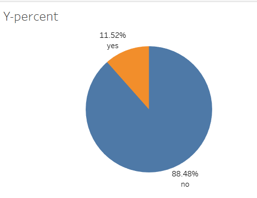
Among all the Y attributes, the majority of customers did not complete their fixed deposit subscription in the end, and over 88% of customers did not choose to subscribe. The remaining 11% of customers chose not to subscribe to fixed deposits, as shown in the following figure.

Data preprocessing

Remove missing values

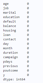
Through the corresponding introduction of the website where the data is located, it can be known that there are no missing values in the corresponding data. After verifying the integrity of the data through code, it is also known that there are no missing values in the attributes of the data.

1	print(bank_data.isnull().sum())

Remove outliers

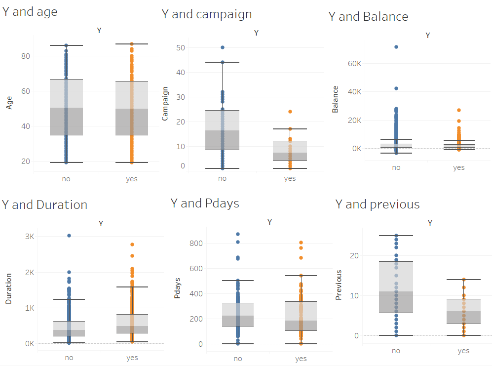
For all non character attributes of continuity in data, through the analysis of the boxplot, we can see that there are many outliers in the four attributes of Campaign, Balance, Duration, and Pdays. Therefore, it is necessary to remove outliers, and the corresponding outliers are shown in the following figure.

Therefore, Python code is used to process the corresponding data with outliers, using 3 σ Method to filter outliers.

def remove_outliers(df, column):
    mean = df[column].mean()
    std = df[column].std()
    df = df[(df[column] > mean - 3 * std) & (df[column] < mean + 3 * std)]
    return df

After processing, the box diagrams for Y and Campaign, Balance, Duration, and Pdays are shown below

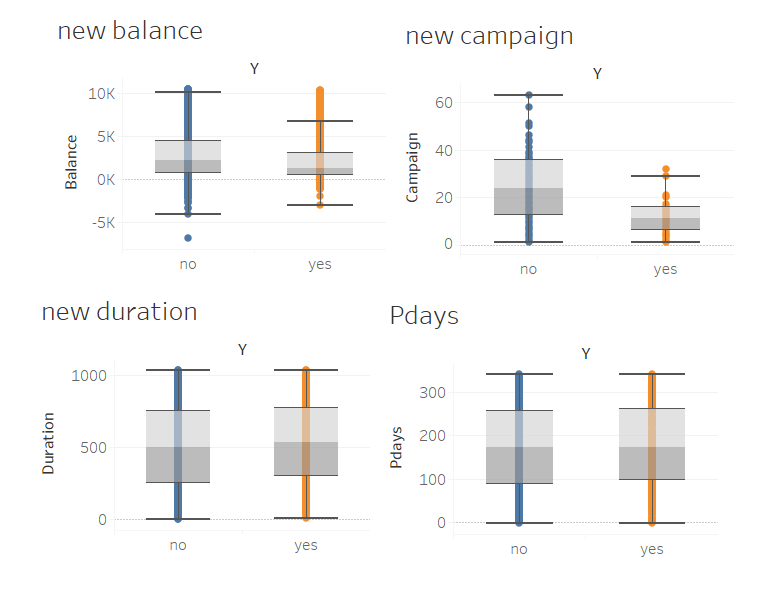
It can be seen that this method has great effectiveness.

Data normalization

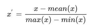
Since all data contains different ranges and not all data can be digitized, we need to normalize the data. Therefore, we need to perform a normalization operation: normalize=lambda x: (x-x.mean())/(x.max() - x.min()) . Namely, mean normalization. Corresponding to the formula shown in the following figure:

Analyze the data

Due to the need for classification methods, all data should be considered, not just numerical data. So we will analyze the relationship between education and loan.Explore the corresponding debt situation at each learning stage, as debt situation has a significant impact on whether to apply for fixed deposits.The relationship between the two is shown in the following figure.

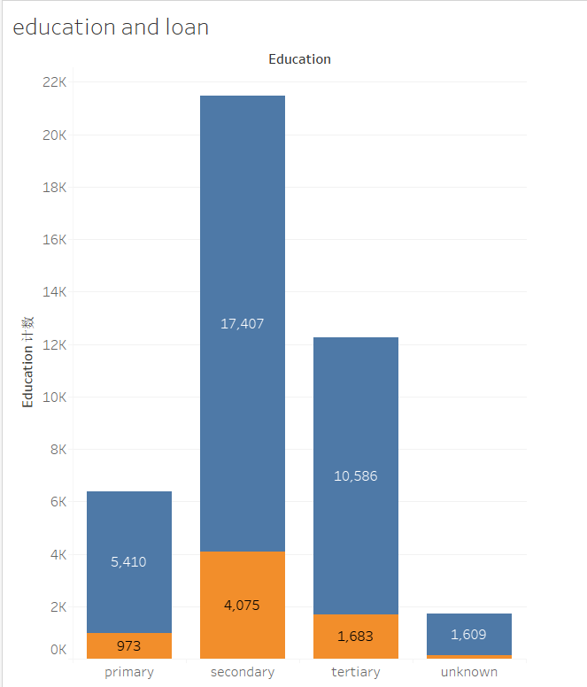
Among them, the number of people with a secondary education background is the highest, and they are easily in debt. Nearly 20% of them still have outstanding loans, while the number of people who choose not to fill in their education background is the lowest, and less than 8% of them have outstanding loans.

When it comes to corresponding liabilities, the relationship between age savings and education cannot be avoided.

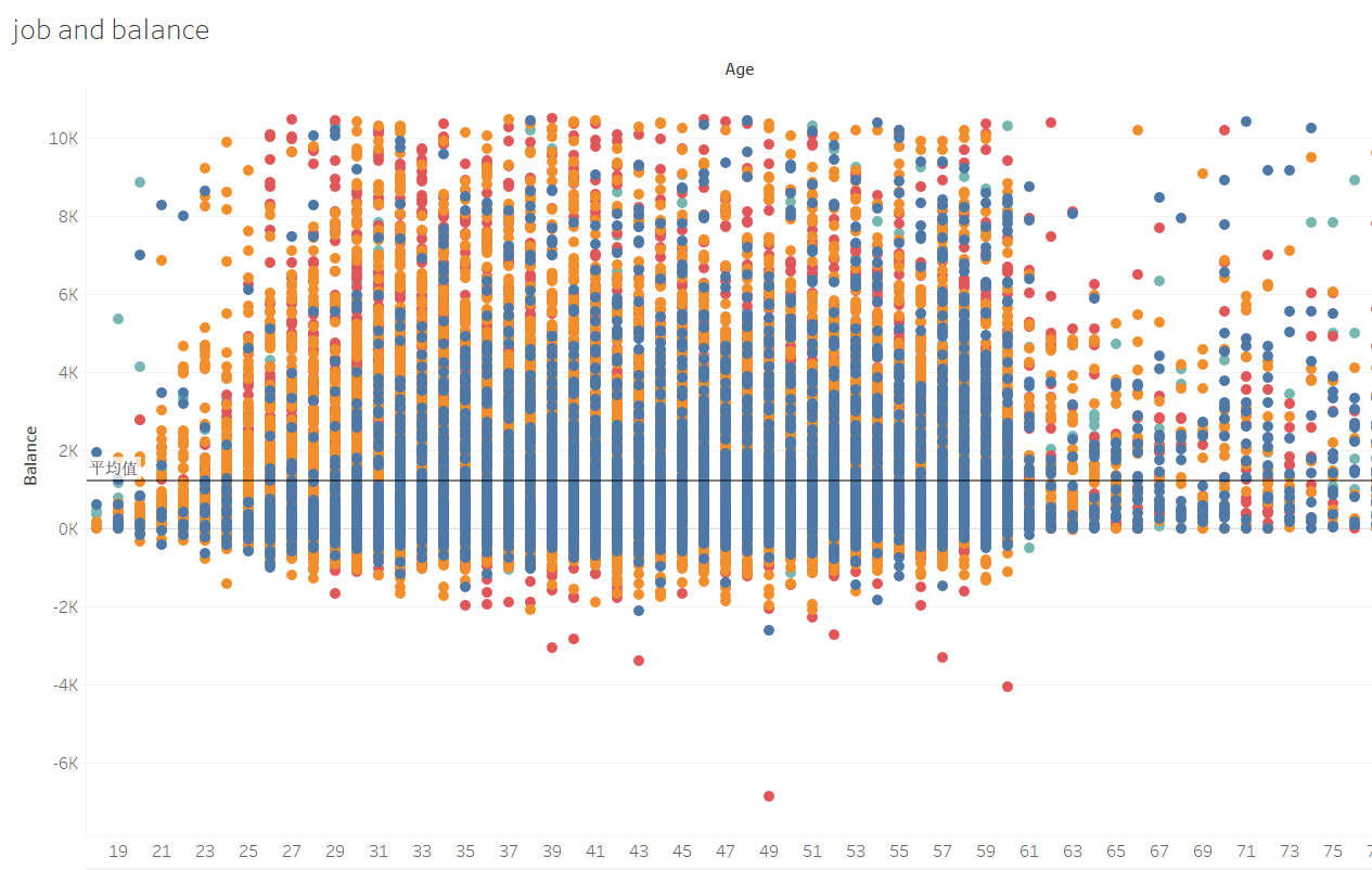
It can be seen that people with a primary school diploma usually have less savings, as the corresponding dataset for primary school is located closer to the X-axis.

summary

Firstly, we analyzed the distribution range of corresponding Y. Afterwards, we analyzed the relationship between the attributes of the numerical part and Y, identified outliers through the corresponding boxplot of the distribution, and utilized 3 σ The method solves the problem of outliers and verifies it. Afterwards, we discovered some simple relationships between education, age, and wage debt.

Assignment 2

Attribute selection

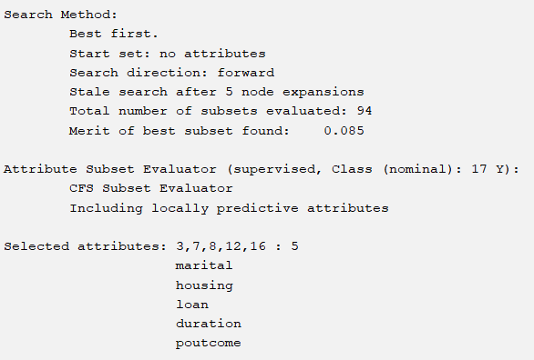
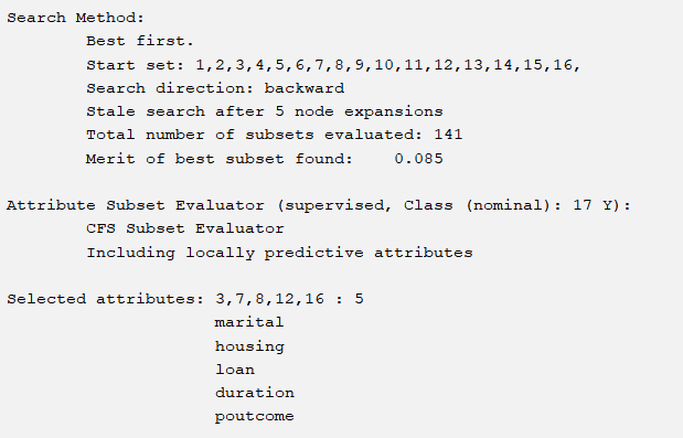
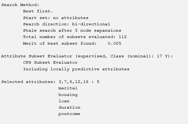
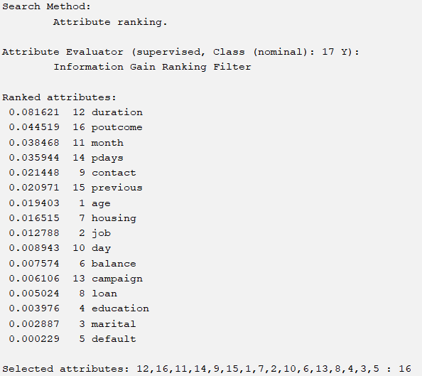
We need to choose several excellent selection methods to select several excellent attributes. If we adopt the importance ranking mechanism for corresponding attributes, we will choose the top five. The following are six corresponding situations. They are respectively

BestFirst+CfsSubsetEval(forward,backward,bi-directional)

Ranker+InfoGainAttributeEval

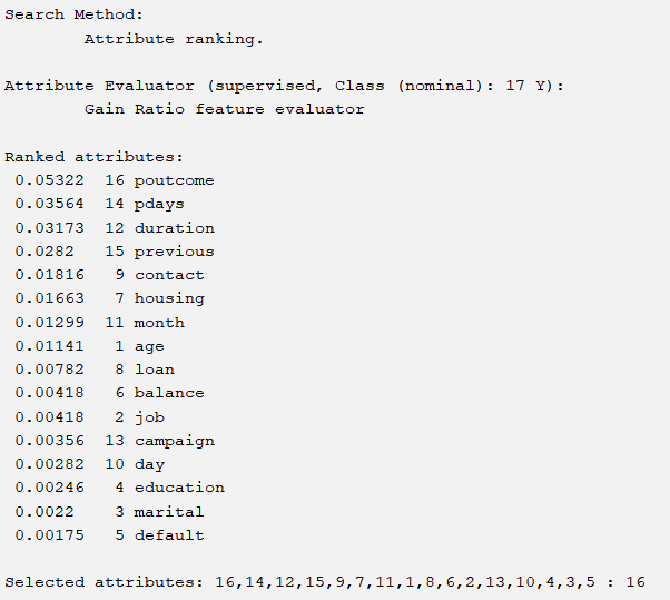
Ranker+GainRatioAttributeEval

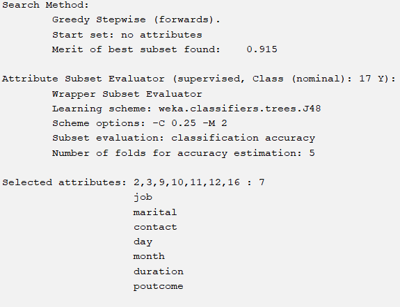
GreedyStepwise+WrapperSubsetEval

And evaluate with J48 with the same parameters

The corresponding six methods have 4 different attribute choices, and the accuracy of J48 corresponding to the same parameter is shown in the table below：

method	accuracy
BestFirst+CfsSubsetEval(forward,backward,bi-directional)	90.8482%
Ranker+InfoGainAttributeEval	91.0979%
Ranker+GainRatioAttributeEval	90.7447 %
GreedyStepwise+WrapperSubsetEval	91.588 %

So our selection method is the last oneGreedyStepwise+WrapperSubsetEval

The final attribute selection is shown in the following table

Attributes	If we choose
age	False
job	True
marital	True
education	False
default	False
balance	False
housing	False
loan	False
contact	True
day	True
month	True
duration	True
campaign	False
pdays	False
previous	False
poutcome	True

Learn scheme

This dataset is only used for classification, and WEKA contains many classification ：method models. We ultimately chose OneR, Naive Bayesian,J48, KNN, and stacking,We ultimately chose an 8:2 ratio between the training and testing sets。

OneR

OneR is the meaning of One Rule, which is a rule that only looks at one feature of a certain thing and then predicts its category (selecting a feature with a low error rate).
By testing the processed dataset, we achieved an accuracy of 90.492%.

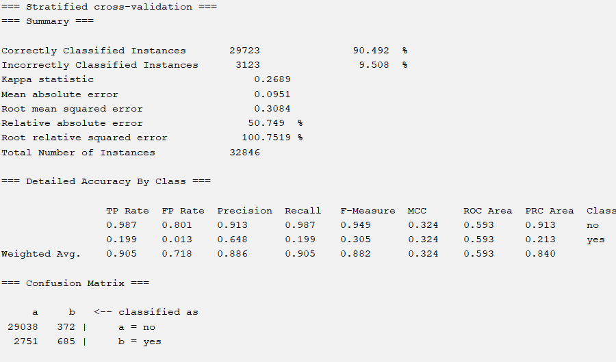
Adjusting minBuchetSize does not change the corresponding accuracy, so the default corresponding result is the optimal OneR result. It can be seen that even the simplest OneR method can achieve significant accuracy.

Naive Bayesian

Naive Bayesian algorithm is one of the most widely used classification algorithms.
The Naive Bayesian method is a simplification of the Bayesian algorithm, which assumes that the attributes are conditionally independent of each other when the target value is given. That is to say, no attribute variable has a significant proportion to the decision result, and no attribute variable has a small proportion to the decision result. Although this simplification approach reduces the classification performance of Bayesian classification algorithms to a certain extent, it greatly simplifies the complexity of Bayesian methods in practical application scenarios.

Algorithm principle

Assumption of characteristic conditionsAssuming there is no connection between each feature, given a training dataset where each sample $x$ all include n-dimensional features，即 $x = ({x_1},{x_2}, \cdots ,{x_n})$ ，Class tag set contains K categories，assume

For a given new sample $x$ ，To determine which category it belongs to, according to Bayesian theorem, one can obtain $x$ belong ${y_k}$ Probability $P({y_k}|x)$

![P({y_k}|x) = \frac