GWAS及其可视化

Association test
Overview

Genetic models
To test the association between a phenotype and genotypes, we need to group the genotypes based on genetic models.
There are three basic genetic models:
为了测试表型和基因型之间的关联,我们需要根据遗传模型对基因型进行分组。
有三种基本的遗传模型:
- Additive model (ADD)加法模型(ADD)
- Dominant model (DOM)主导模型(DOM)
- Recessive model (REC)隐性模型(REC)
info “Three genetic models”信息“三种遗传模型”
For example, suppose we have a biallelic SNP whose reference allele is A and the alternative allele is G.
例如,假设我们有一个双等位基因SNP,其参考等位基因是A,替代等位基因为G。
There are three possible genotypes for this SNP: AA, AG, and GG.

This table shows how we group different genotypes under each genetic model for association tests using linear or logistic regressions.

|Genetic models|AA|AG|GG|
|-|-|-|-|
|Additive model|0|1|2|按照替代等位基因的数目进行分类
|Dominant model|0|1|1|存在突变基因就为1
|Recessive model|0|0|1|两个基因全部突变才为1
info “Contingency table and non-parametric tests”
info“应急表和非参数测试”
A simple way to test association is to use the 2x2 or 2x3 contingency table. For dominant and recessive models, Chi-square tests are performed using the 2x2 table. For the additive model, Cochran-Armitage trend tests are performed for the 2x3 table. However, the non-parametric tests do not adjust for the bias caused by other covariates like sex, age and so forth.
测试关联的一个简单方法是使用2x2或2x3列联表。对于显性和隐性模型,使用2x2表进行卡方检验。对于加性模型,对2x3表进行了Cochran-Armitage趋势检验。然而,非参数检验并没有调整由性别、年龄等其他协变量引起的偏差。

Association testing basics
For quantitative traits, we can employ a simple linear regression model to test associations:对于数量性状,我们可以使用一个简单的线性回归模型来检验关联:
-
 is the genotype matrix.是基因型矩阵。
 is the effect size for variants.是变体的效果大小。
 and
and  are covariates and their effects.是协变量及其影响。
- e is the error term.是误差项。
info “Interpretation of linear regression”

For binary traits, we can utilize the logistic regression model to test associations:
对于二元性状,我们可以利用逻辑回归模型来检验关联:

info “Linear regression and logistic regression”
info“线性回归和逻辑回归” 
File Preparation
To perform genome-wide association tests, usually, we need the following files:
为了进行全基因组关联测试,我们通常需要以下文件:
Genotype file (or dosage file) : usually in PLINK format, VCF format, or BGEN format.
基因型文件(或剂量文件):通常为PLINK格式、VCF格式或BGEN格式。
Phenotype file : plain text file.
表型文件:纯文本文件。
Covariate file (optional): plain text file. Commonly used covariates include age, sex, and top Principal Components.
协变量文件(可选):纯文本文件。常用的协变量包括年龄、性别和主要成分。
example “Phenotype and covariate files”
示例“表型和协变量文件”
1 | Phenotype file for a simulated binary trait; B1 is the phenotype name; 1 means the control, 2 means the case. |
Association tests using PLINK
Please check https://www.cog-genomics.org/plink/2.0/assoc for more details.
请检查https://www.cog-genomics.org/plink/2.0/assoc了解更多详情。
We will perform logistic regression with firth correction for a simulated binary trait under the additive model using the 1KG East Asian individuals.
我们将使用1KG East Asian individuals在ADD模型下对模拟的二元性状进行带有Firth校正的逻辑回归。
note “Firth 校正”
Adding a penalty term to the log-likelihood function when fitting the logistic model results in less bias. - Firth, David. “Bias reduction of maximum likelihood estimates.” Biometrika 80.1 (1993): 27-38.
在拟合逻辑模型时,在对数似然函数中添加惩罚项可以减少偏差。”Bias reduction of maximum likelihood estimates.” Biometrika 80.1 (1993): 27-38.
note “Quantitative traits”注“数量性状”
For quantitative traits, linear regressions will be performed and in this case, we do not need to add firth (since Firth correction is not appliable).
对于数量性状,将进行线性回归,在这种情况下,我们不需要添加“”(Firth)因为Firth校正不适用)。
!!! example “Sample codes for association test using plink for binary traits”
 1
2
3
4
5
6
7
8
9
10
11
12
13
14
15
16
17
18
genotypeFile="../04_Data_QC/sample_data.clean" # the clean dataset we generated in previous section
phenotypeFile="../01_Dataset/1kgeas_binary.txt" # the phenotype file
covariateFile="../05_PCA/plink_results_projected.sscore" # the PC score file
covariateCols=6-10
PC1,PC2另作他用
colName="B1"
threadnum=2
下面有这段代码的具体解释
plink2 \
	--bfile ${genotypeFile} \
	--pheno ${phenotypeFile} \
	--pheno-name ${colName} \
	--maf 0.01 \
	--covar ${covariateFile} \
	--covar-col-nums ${covariateCols} \
	--glm hide-covar firth  firth-residualize single-prec-cc \
	--threads ${threadnum} \
	--out 1kgeas
note
Using the latest version of PLINK2, you need to add firth-residualize single-prec-cc to generate the results. (The algorithm and precision have been changed since 2023 for firth regression)
使用最新版本的PLINK2,您需要添加firth-residualize single-prec-cc以生成结果。(自2023年以来,firth 回归的算法和精度发生了变化)
You will see a similar log like:
您将看到类似的日志:
1 | !!! example "Log" |
Let’s check the first lines of the output:
!!! example “Association test results”
1
2
3
4
5
6
7
8
9
10
#CHROM POS ID REF ALT PROVISIONAL_REF? A1 OMITTED A1_FREQ TEST OBS_CT OR LOG(OR)_SE Z_STAT P ERRCODE
1 15774 1:15774:G:A G A Y A G 0.0282828 ADD 495 NA NA NA NA FIRTH_CONVERGE_FAIL
1 15777 1:15777:A:G A G Y G A 0.0737374 ADD 495 NA NA NA NA FIRTH_CONVERGE_FAIL
1 57292 1:57292:C:T C T Y T C 0.104675 ADD 492 NA NA NA NA FIRTH_CONVERGE_FAIL
1 77874 1:77874:G:A G A Y A G 0.0191532 ADD 496 1.12228 0.46275 0.249299 0.80313 .
1 87360 1:87360:C:T C T Y T C 0.0231388 ADD 497 NA NA NA NA FIRTH_CONVERGE_FAIL
1 125271 1:125271:C:T C T Y C T 0.0292339 ADD 496 1.53387 0.373358 1.1458 0.25188 .
1 232449 1:232449:G:A G A Y A G 0.185484 ADD 496 0.884097 0.168961 -0.729096 0.465943 .
1 533113 1:533113:A:G A G Y G A 0.129555 ADD 494 0.90593 0.196631 -0.50243 0.615365 .
1 565697 1:565697:A:G A G Y G A 0.334677 ADD 496 1.04653 0.15286 0.297509 0.766078 .
info “Usually, other options are added to enhance the sumstats”
info“通常,会添加其他选项来增强sumstats”
* --keep xxx/kiso2021/for_plink2/unrelated.sample.id	# Because the standard linear     regression does not account for the relatedness, the kinship-pruned samples in last steps are suggested.
* --mach-r2-filter 0.7 2.0	# It allows to use only the variants passed an (MaCH)Rsq filter.  NOTE: when pgen file is used, the upper boundary should be 2.
* --glm **cols=+a1freq,+machr2** firth-fallback **omit-ref**	# The `cols=` requests the  following columns in the sumstats: here are allele1 frequency and (MaCH)Rsq, `firth-fallback`     will test the common variants without firth correction, which could improve the speed,     `omit-ref` will force the ALT==A1==effect allele, otherwise the minor allele would be tested     (see the above result, which ALT may not equal A1).
* --covar-variance-standardize	# To normalize the covariates which may at a huge scale, like     AGE**AGE.
* --covar-name AGE SEX PC1-PC20	# Instead of setting the index of columns, directly specify the     column name.
(optional)Genomic control
Genomic control (GC) is a basic method for controlling for confounding factors including population stratification.
基因组控制(GC)是控制包括群体分层在内的混杂因素的基本方法。
We will calculate the genomic control factor (lambda GC) to evaluate the inflation. The genomic control factor is calculated by dividing the median of observed Chi square statistics by the median of Chi square distribution with the degree of freedom being 1 (which is approximately 0.455).
我们将计算基因组控制因子(λGC)来评估膨胀。基因组控制因子是通过将观察到的卡方统计量的中值除以卡方分布的中值来计算的,自由度为1(约为0.455)。

Then, we can used the genomic control factor to correct observed Chi suqare statistics.
然后,我们可以使用基因组控制因子来校正观察到的Chi-suqare统计数据。

Genomic inflation is based on the idea that most of the variants are not associated, thus no deviation between the observed and expected Chi square distribution, except the spikes at the end. However, if the trait is highly polygenic, this assumption may be violated.
基因组膨胀基于这样一种观点,即大多数变异都没有关联,因此除了末端的尖峰外,观察到的卡方分布和预期的卡方分配之间没有偏差。然而,如果该性状是高度多基因的,则可能会违反这一假设。
Reference: Devlin, B., & Roeder, K. (1999). Genomic control for association studies. Biometrics, 55(4), 997-1004.
(optional)Significant loci
Please check Visualization using gwaslab
Loci that reached genome-wide significance threshold (P value < 5e-8) :
达到全基因组显著性阈值的位点(P值<5e-8):-log10(p)>-log(5e-8)
1 | SNPID CHR POS EA NEA EAF SE Z P OR N STATUS REF ALT |
warning
This is just to show the analysis pipeline and data format. The trait was simulated under an unreal condition (effect sizes are extremely large) so the result is meaningless here.
这只是为了显示分析管道和数据格式。该特征是在不真实的条件下模拟的(效果大小非常大),因此结果在这里毫无意义。
info “Allele frequency and Effect size”
info“等位基因频率和效应大小” 
Visualization
To visualize the sumstats, we will create the Manhattan plot, QQ plot and regional plot.
为了可视化sumstats,我们将创建曼哈顿图、QQ图和区域图。
Please check for codes : Visualization using gwaslab

Manhattan plot
Manhattan plot is the most classic visualization of GWAS summary statistics. It is a form of scatter plot. Each dot represents the test result for a variant. variants are sorted by their genome coordinates and are aligned along the X axis. Y axis shows the -log10(P value) for tests of variants in GWAS.
曼哈顿图是GWAS汇总统计中最经典的可视化。这是散点图的一种形式。每个点代表一个变体的测试结果。变体按其基因组坐标排序,并沿X轴排列。Y轴显示了GWAS中变体测试的-log10(P值)。
note
This kind of plot was named after Manhattan in New York City since it resembles the Manhattan skyline.
这种地块以纽约市曼哈顿的名字命名,因为它类似于曼哈顿的天际线。
info “A real Manhattan plot”“真正的曼哈顿图表”

The autor took this photo in 2020 just before the COVID-19 pandemic. It was a cloudy and misty day. Those birds formed a significance threshold line. And the skyscrapers above that line resembled the significant signals in your GWAS. I believe you could easily get how the GWAS Manhattan plot was named.
作者在2020年新冠肺炎大流行前拍下了这张照片。那是一个多云多雾的日子。这些鸟形成了一条重要的阈值线。那条线上方的摩天大楼就像你们GWAS中的重要信号。我相信你很容易就能知道GWAS曼哈顿地块是如何命名的。
Data we need from sumstats to create Manhattan plots:
我们需要来自sumstats的数据来创建曼哈顿图:
- Chromosome
- Basepair position
- P value or -log10(P)
tips “Steps to create Manhattan plot”
1. sort the variants by genome coordinates.
2. map the genome coordinates of variants to the x axis.
3. convert P value to -log10(P).
4. create the scatter plot.
1.按基因组坐标对变异进行排序。
2.将变异的基因组坐标映射到x轴。
3.将P值转换为-log10(P)。
4.绘制散点图。
Quantile-quantile plot
Quantile-quantile plot (also known as Q-Q plot), is commonly used to compare an observed distribution with its expected distribution. For a specific point (x,y) on Q-Q plot, its y coordinate corresponds to one of the quantiles of the observed distribution, while its x coordinate corresponds to the same quantile of the expected distribution.
分位数-分位数图(也称为Q-Q图)通常用于比较观察到的分布与其预期分布。对于Q-Q图上的特定点(x,y),其y坐标对应于观察到的分布的分位数之一,而其x坐标对应于预期分布的相同分位数。预期分布应当是从最小值(-log(0.01),最大值-log(1/样例数)
-log()大于2的才算是明显的可以用来计算的位点
Quantile-quantile plot is used to check if there is any significant inflation in P value distribution, which usually indicates population stratification or cryptic relatedness.
分位数-分位数图用于检查P值分布是否存在显著膨胀,这通常表明人口分层或隐性相关性。
Data we need from sumstats to create the Manhattan plot:
我们需要来自sumstats的数据来创建曼哈顿图:
- P value or -log10(P)
tips “Steps to create Q-Q plot”
Suppose we have `n` variants in our sumstats,

1. convert the `n` P value to -log10(P).
2. sort the -log10(P) values in asending order.
3. get `n` numbers from `(0,1)` with equal intervals.
4. convert the `n` numbers to -log10(P) and sort in ascending order.
4. create scatter plot using the sorted -log10(P) of sumstats as Y and sorted -log10(P) we generated as X.
假设我们的sumstats中有n个变量,
1.将'n'P值转换为-log10(P)。
2.按顺序对-log10(P)值进行排序。
3.以相等的间隔从“(0,1)”中得到“n”个数字。
4.将“n”数字转换为-log10(P),并按升序排序。
4.使用sumstats的sorted-log10(P)作为Y,使用我们生成的sorted-log10(P)作为X,创建散点图。
note
The expected distribution of P value is a Uniform distribution from 0 to 1.
P值的预期分布是从0到1的均匀分布。但实际上不用取那么多的结果

Regional plot
Manhattan plot is very useful to check the overview of our sumstats. But if we want to check a specific genomic locus, we need a plot with finer resolution. This kind of plot is called a regional plot. It is basically the Manhattan plot of only a small region on the genome, with points colored by its LD r2 with the lead variant in this region.
曼哈顿图对于查看我们的sumstats概览非常有用。但如果我们想检查特定的基因组位点,我们需要一个分辨率更高的图。这种情节被称为区域情节。它基本上是基因组上只有一个小区域的曼哈顿图,其点由LD r2着色,该区域有前导变体。
Such a plot is especially helpful to understand the signal and loci, e.g., LD structure, independent signals, and genes.
这样的图对于理解信号和位点特别有帮助,例如LD结构、独立信号和基因。
The regional plot for the loci of 2:55513738:C:T.
Please check Visualization using gwaslab

(optional)GWAS-SSF
To standardize the format of GWAS summary statistics for sharing, GWAS-SSF format was proposed in 2022. This format is now used as the standard format for GWAS Catalog.
为了规范GWAS汇总统计数据的共享格式,2022年提出了GWAS-SSF格式。此格式现在用作GWAS目录的标准格式。
GWAS-SSF由以下部分组成:
GWAS-SSF consists of :
- a tab-separated data file with well-defined fields (shown in the following figure)
- an accompanying metadata file describing the study (such as sample ancestry, genotyping method, md5sum, and so forth)
example “Schematic representation of GWAS-SSF data file”

plink2
–bfile ${genotypeFile}
–pheno ${phenotypeFile}
–pheno-name ${colName}
–maf 0.01
–covar ${covariateFile}
–covar-col-nums ${covariateCols}
–glm hide-covar firth firth-residualize single-prec-cc
–threads ${threadnum}
–out 1kgeas
PLINK2 基因数据分析代码解释
以下代码用于执行基于广义线性模型(GLM)的基因-表型关联分析,使用 Firth 回归校正和协变量调整:
1 | plink2 --bfile ${genotypeFile} \ |
一、输入文件说明
基因型文件 (
--bfile ${genotypeFile})- 格式:PLINK 二进制格式(
.bed/.bim/.fam三文件组) - 内容:
.bed:样本基因型数据(二进制).bim:SNP 位点信息(染色体、位置、等位基因等).fam:样本基础信息(个体 ID、家系 ID 等)
- 示例:
HapMap_3_r3_11
- 格式:PLINK 二进制格式(
表型文件 (
--pheno ${phenotypeFile})- 格式:文本文件(如 TSV/CSV),需包含样本 ID 列和表型值列
- 要求:
- 表型可为连续型(如血压值)或二元型(如病例/对照用 1/0 表示)
- 缺失值需用特定字符标记(如
NA)
- 引用:需与基因型文件的样本 ID 匹配
表型列名 (
--pheno-name ${colName})- 指定表型文件中目标分析列的名称(如
height或disease_status)
- 指定表型文件中目标分析列的名称(如
协变量文件 (
--covar ${covariateFile})- 格式:文本文件,每行为一个样本的协变量数据
- 内容:可包含年龄、性别、主成分(PCA 结果)等调整变量
- 引用:需事先通过 PLINK 或
sgkit生成
协变量列号 (
--covar-col-nums ${covariateCols})- 指定协变量文件中使用的列索引(从 1 开始),如
3,5,6-8
- 指定协变量文件中使用的列索引(从 1 开始),如
二、关键参数解析
| 参数 | 作用 | 示例值/说明 |
|---|---|---|
--maf 0.01 |
过滤最小等位基因频率(MAF) 排除 MAF < 1% 的 SNP |
质量控制常用阈值 |
--glm |
启用广义线性模型分析 | 支持线性/逻辑回归 |
hide-covar |
输出中隐藏协变量结果 | 仅保留 SNP 关联统计量 |
firth |
启用 Firth 偏倚校正 | 解决病例-对照数据中的分离问题 |
firth-residualize |
对协变量进行 Firth 残差化 | 增强数值稳定性 |
single-prec-cc |
病例-对照分析使用单精度浮点 | 加速计算 |
--threads ${threadnum} |
指定并行计算线程数 | 提升大样本分析速度 |
三、输出文件说明
输出前缀 1kgeas 将生成以下文件:
主要结果文件:
1kgeas.<phenotype>.glm.<model>- 内容(每行一个 SNP 的关联分析结果):
1
2
#CHROM POS ID REF ALT A1 TEST OBS_CT BETA SE P
1 12345 rs123 A G G ADD 1000 0.12 0.05 0.016 - 列含义:
BETA:效应值(连续表型为斜率,二元表型为 log(OR))SE:标准误P:关联显著性 p 值
- 内容(每行一个 SNP 的关联分析结果):
日志文件:
1kgeas.log- 记录分析过程、样本/SNP 数量、警告或报错信息
四、分析流程特点
- 质量控制:通过
--maf过滤低频 SNP,提高结果可靠性 - 协变量控制:校正混杂因素(如人群结构)
- 算法优化:
- Firth 校正解决小样本偏倚问题
- 单精度计算加速病例-对照分析
- 高效计算:多线程处理大规模基因数据
PLINK2命令生成的显著相关性P值解释
在PLINK2中,当您使用命令(如--glm、--linear或--logistic)进行遗传关联分析时,输出的P值用于评估单核苷酸多态性(SNP)与表型之间相关性的统计显著性。针对您的问题:P值越大,并不表示更相关于某一表型;相反,P值越小,表示相关性越显著。 下面我将逐步解释原因,并澄清常见误解。
1. P值的含义和解释
P值的定义:在假设检验中,P值代表在零假设(null hypothesis)成立的条件下,观察到当前数据(或更极端数据)的概率。对于相关性分析:
零假设
 :SNP与表型无关联(即效应大小
  )。
)。备择假设
 :SNP与表型有关联(
 )。
)。P值计算公式为:

P值与相关性的关系:
- P值小(例如
 ):表示有强证据拒绝零假设,支持SNP与表型存在显著相关性。
 - P值大(例如
 ):表示数据不足以拒绝零假设,即没有显著证据支持相关性;这通常意味着SNP与表型的关联很弱或不存在。
 - 因此,P值衡量的是统计显著性的强度,而非相关性的方向或大小。例如,P值接近0.8表示相关性不显著,而P值接近0.001表示高度显著。
- P值小(例如
在PLINK2的输出中,P值通常列在P列(如--glm命令生成的.glm.linear文件)。您应结合效应大小(如回归系数  或OR值)来全面评估相关性:
- **效应大小(例如
 )**:表示相关性的方向和强度(正相关或负相关,值越大表示影响越强)。
 - P值:仅表示这种效应是否统计显著。
混淆P值和效应大小是常见错误:高P值可能对应于弱效应或噪声,而低P值才表示可靠的相关性。
2. 在PLINK2中的具体应用
常用命令:PLINK2的
--glm命令常用于线性或逻辑回归分析,生成P值。例如:1
plink2 --bfile mydata --pheno pheno.txt --glm --out results
输出文件(如
results.glm.linear)包含列:ID(SNP标识),BETA(效应大小),P(P值)。输出示例:
ID BETA P rs1234 0.25 0.003 rs5678 -0.10 0.75 - 这里,rs1234的P值小(0.003),表示与表型显著相关;rs5678的P值大(0.75),表示无显著关联。
注意事项:
- PLINK2的P值基于标准统计检验(如Wald test)。P值阈值通常设为0.05或更严格(如5e-8用于基因组宽关联研究)。
- P值受样本大小和效应大小影响:大样本可能使弱效应也产生小P值,反之亦然。
3. 为什么P值越大不表示更相关?
P值本质上是一个概率指标,并非相关性的直接度量。相关性的强度由效应大小(如 $\beta$ 或相关系数 $r$)决定。
- 例如,在回归模型中,
 值大且P值小,表示强相关。
 - 如果P值大,即使
 值看似大,也可能由于随机变异(如小样本噪声)导致,不可靠。
- 例如,在回归模型中,
数学说明:假设一个简单线性模型
 ,其中
,其中  是表型,
是表型, 是基因型。检验
的P值计算为:

其中
 是估计效应大小,
 是标准误,
是标准误, 是标准正态分布函数。P值随
  增大而减小,表明只有效应大且变异小时P值才小。
总之,在PLINK2分析中,P值越小,相关性越显著;P值越大,相关性越不显著。务必与效应大小结合解读,避免误解。
python可视化代码(不使用gwaslab)
1 | import pandas as pd |
1 | gwas_results |
| #CHROM | POS | ID | REF | ALT | PROVISIONAL_REF? | A1 | OMITTED | A1_FREQ | TEST | OBS_CT | OR | LOG(OR)_SE | Z_STAT | P | ERRCODE | |
|---|---|---|---|---|---|---|---|---|---|---|---|---|---|---|---|---|
| 0 | 1 | 15774 | 1:15774:G:A | G | A | Y | A | G | 0.028283 | ADD | 495 | 0.745933 | 0.394259 | -0.743467 | 0.457199 | . |
| 1 | 1 | 15777 | 1:15777:A:G | A | G | Y | G | A | 0.073737 | ADD | 495 | 0.839657 | 0.250121 | -0.698707 | 0.484735 | . |
| 2 | 1 | 57292 | 1:57292:C:T | C | T | Y | T | C | 0.104675 | ADD | 492 | 1.101050 | 0.215278 | 0.447152 | 0.654766 | . |
| 3 | 1 | 77874 | 1:77874:G:A | G | A | Y | A | G | 0.019153 | ADD | 496 | 1.122270 | 0.462750 | 0.249279 | 0.803145 | . |
| 4 | 1 | 87360 | 1:87360:C:T | C | T | Y | T | C | 0.023139 | ADD | 497 | 1.673520 | 0.439532 | 1.171540 | 0.241382 | . |
| ... | ... | ... | ... | ... | ... | ... | ... | ... | ... | ... | ... | ... | ... | ... | ... | ... |
| 1128727 | 22 | 51217954 | 22:51217954:G:A | G | A | Y | A | G | 0.033199 | ADD | 497 | 0.697307 | 0.362169 | -0.995476 | 0.319505 | . |
| 1128728 | 22 | 51218377 | 22:51218377:G:C | G | C | Y | C | G | 0.033333 | ADD | 495 | 0.697540 | 0.362213 | -0.994432 | 0.320013 | . |
| 1128729 | 22 | 51218615 | 22:51218615:T:A | T | A | Y | A | T | 0.033266 | ADD | 496 | 0.688624 | 0.362476 | -1.029200 | 0.303386 | . |
| 1128730 | 22 | 51222100 | 22:51222100:G:T | G | T | Y | T | G | 0.039157 | ADD | 498 | 1.221010 | 0.323176 | 0.617870 | 0.536661 | . |
| 1128731 | 22 | 51239678 | 22:51239678:G:T | G | T | Y | T | G | 0.034137 | ADD | 498 | 1.227610 | 0.354398 | 0.578647 | 0.562827 | . |
1128732 rows × 16 columns
1 | #数据预处理 |
Loaded 1128732 SNPs with association results
1 | def plot_manhattan(gwas_df, skip,title="GWAS Manhattan Plot"): |


使用tableau的可视化结果(带标记)

1 | expected = (-np.log10(np.linspace(1/8510, 0.01, 8510))) |
array([3.92992956, 3.92565822, 3.92142848, …, 2.00010089, 2.00005044,
2. ], shape=(8510,))
1 | def plot_qq(gwas_df, skip, title="GWAS Q-Q Plot"): |

tableau:
1 | def plot_regional(gwas_df, chrom, start, end, title="Regional Association Plot"): |

总览